public_data_path = 'public_data/' # make sure the folder has this name or change it3. Create submissions
In this notebook we will explore the datasets of the AnDi 2 challenge and show how to properly create a submission. We will consider that you have already read the paper and know the basics of the challenge. This notebook has three sections:
- Reading videos and trajectories: the public data - we will show how the public data looks like, which is the one used to make the predictions.
- Creating and submitting predictions - we will generate some trivial predictions for the previous data and illustrate the structure of a submission.
- Work on your own datasets - we will show how to read the Starting Kit, generate new datasets with the
andi_datasetslibrary and score your data locally.
Reading videos and trajectories: the public data
First things first: you need to download the public data to perform the predictions available in the competition’s Codalab webpage (link not yet available). We will showcase here how to do so in the Development phase data. For that, go to the competition, then Participate > Files and download the Public Data for Phase #1 Development. Once unzipped, the dataset should have the following file structure:
public_dat
│
└─── track_1 (videos)
| │
| └─── exp_Y
│ │
│ └─── videos_fov_X.tiff (video for each fov)
│
│
└─── track_2 (trajectories)
│
└─── exp_Y
│
└─── traj_fov_X.csv (trajectories for each FOV) where Y goes from 0 to 9 and X from 0 to 29. This means that we have 10 experiments with 30 FOVs each.
Track 1: videos
Track 1 focuses on videos. Each of the tiffs contains a video mimicking a typical single particle tracking experiment (see the paper for details). Let’s load one of the videos. You can do so with the following function:
from andi_datasets.utils_videos import import_tiff_video
import matplotlib.pyplot as plt
import numpy as np
np.random.seed(0)
video = import_tiff_video(public_data_path+'track_1/exp_0/videos_fov_1.tiff')The first frame contains the label of the VIP particles. The pixel indicates the initial position of the particle and the value provides the particle’s index.
VIP particles are the ones you will need to characterize in the single trajectory task (see more on this below).
plt.matshow(video[0])
plt.xlabel('pixel');plt.ylabel('pixel');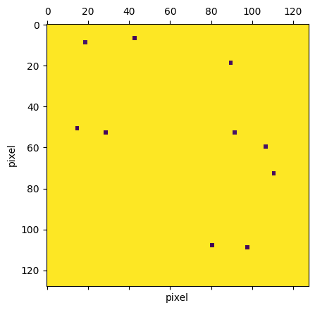
To access the indices of the VIP particles, take the unique values of the initial frame:
np.unique(video[0])array([ 16, 18, 19, 20, 21, 22, 24, 27, 28, 29, 255], dtype=uint8)From the previous numbers, 255 is the background and the rest are the indices of the VIP particles.
We can visualize the videos with the built-in function play_video.
from andi_datasets.utils_videos import play_videoLet’s see how the video looks like! play_video expects an object with shape (num_frames, pixels, pixels, channels). In this case, we will need to add an additional axis for the channels (grayscale).
You may need to install
pillow(simplypip install pillow) to play the following video.
play_video(video[1:,:,:,np.newaxis])As you can see, there many more particles besides the VIP particles. These will help you find the ensemble properties of the experiment (more on this below).
Track 2: trajectories
Track 2 focuses on trajectories, as we did in the previous challenge. The trajectories come in a csv file with four columns: - traj_idx: index of the trajectory - frame: frame at which each of the time steps was recorded - x and y: pixel x and y position.
Let’s look at the data:
import pandas as pd
df = pd.read_csv(public_data_path+'track_2/exp_0/trajs_fov_0.csv')
df| traj_idx | frame | x | y | |
|---|---|---|---|---|
| 0 | 0.0 | 0.0 | 93.654332 | 104.089646 |
| 1 | 0.0 | 1.0 | 93.602970 | 103.040118 |
| 2 | 0.0 | 2.0 | 94.925046 | 104.376142 |
| 3 | 0.0 | 3.0 | 93.559753 | 102.780234 |
| 4 | 0.0 | 4.0 | 92.713807 | 102.126589 |
| ... | ... | ... | ... | ... |
| 4429 | 25.0 | 195.0 | 179.430772 | 132.665685 |
| 4430 | 25.0 | 196.0 | 175.963130 | 130.836672 |
| 4431 | 25.0 | 197.0 | 177.304783 | 129.842511 |
| 4432 | 25.0 | 198.0 | 176.402691 | 131.515115 |
| 4433 | 25.0 | 199.0 | 175.538531 | 132.183690 |
4434 rows × 4 columns
Similar to the previous example, the trajectory indices can be obtained with:
traj_idx = df.traj_idx.unique()The data for each trajectory can be accessed by masking over the trajectory index.
idx = 0
mask = df.traj_idx == idx
traj = df[mask]traj| traj_idx | frame | x | y | |
|---|---|---|---|---|
| 0 | 0.0 | 0.0 | 93.654332 | 104.089646 |
| 1 | 0.0 | 1.0 | 93.602970 | 103.040118 |
| 2 | 0.0 | 2.0 | 94.925046 | 104.376142 |
| 3 | 0.0 | 3.0 | 93.559753 | 102.780234 |
| 4 | 0.0 | 4.0 | 92.713807 | 102.126589 |
| ... | ... | ... | ... | ... |
| 195 | 0.0 | 195.0 | 89.878535 | 101.287746 |
| 196 | 0.0 | 196.0 | 89.408663 | 101.777232 |
| 197 | 0.0 | 197.0 | 91.881616 | 102.291826 |
| 198 | 0.0 | 198.0 | 91.168064 | 102.299316 |
| 199 | 0.0 | 199.0 | 89.729272 | 104.437141 |
200 rows × 4 columns
Creating and submitting predictions
Now that you know how to read the data, let’s make some predictions! For the sake of this tutorial, we will generate dummy data to populate a fake submission file. The submission file must be structured as follows:
PATH
│
└─── track_1
| │
| └─── exp_Y
│ │
│ └─── fov_X.txt
│ │
│ └─── ensemble_labels.txt
│
│
└─── track_2
│
└─── exp_Y
│
└─── fov_X.txt
│
└─── ensemble_labels.txtThe fov_X.txt files contain the individual predictions for each FOV: every VIP particle in track 1, and every single trajectory in track 2. The ensemble_labels.txt contains the predictions at the ensemble level for the whole experiment.
In our case, we will gather our submission files in the following root path:
import os
path_results = 'res/'
if not os.path.exists(path_results):
os.makedirs(path_results)Important: You can choose to which track / task you want to participate. For example:
-> If you want to focus on Track 1, your submission only needs to contain the folder track_1.
-> If you want to focus on the Ensemble task, the folders only need to contain the ensemble_labels.txt file (no fov_X.txt needed)
Ensemble task
In the ensemble task, you must provide the diffusive properties of each state present in the dataset. The submission file should have the following structure:
| model: modelXXX; | num_state: YYY | ||
|---|---|---|---|
| \(\mu_\alpha^1\); | \(\mu_\alpha^2\); | \(\mu_\alpha^3\); | … |
| \(\sigma_\alpha^1\); | \(\sigma_\alpha^2\); | \(\sigma_\alpha^3\); | … |
| \(\mu_K^1\); | \(\mu_K^2\); | \(\mu_K^3\); | … |
| \(\sigma_K^1\); | \(\sigma_K^2\); | \(\sigma_K^3\); | … |
| \(N_1\); | \(N_2\); | \(N_3\); | … |
The first row contains the diffusion model prediction for the experiment and the number of diffusive states. Below, every column contains the properties for each of the predicted diffusive states:
- \(\mu_\alpha^i\), \(\sigma_\alpha^i\): mean and variance of the anomalous diffusion exponent.
- \(\mu_K^i\), \(\sigma_K^i\): mean and variance of the diffusion coefficient.
- \(N_i\): relative weight of the state (e.g. time spent in it).
It is important to use ; as delimiter of the file.
For the model prediction, the available diffusion models are (and should be written as):
from andi_datasets.datasets_phenom import datasets_phenom
datasets_phenom().avail_models_name['single_state',
'multi_state',
'immobile_traps',
'dimerization',
'confinement']Both \(\alpha\) and \(D\) are bound to some minimal and maximal values:
from andi_datasets.models_phenom import models_phenom
print(f' Min, max D: {models_phenom().bound_D}\n',
f'Min, max alpha: {models_phenom().bound_alpha}') Min, max D: [1e-12, 1000000.0]
Min, max alpha: [0, 1.999]The state weights DO NOT need to be normalized, the scoring program will take care of normalizing by dividing each weight \(N_i\) by their sum (i.e., \(\sum_i N_i\)).
Let’s create a dummy submission. For each track (1 and 2) and experiment (10 in this example), we will create a file with two states and random parameters:
for track in [1,2]:
# Create the folder of the track if it does not exists
path_track = path_results + f'track_{track}/'
if not os.path.exists(path_track):
os.makedirs(path_track)
for exp in range(10):
# Create the folder of the experiment if it does not exits
path_exp = path_track+f'exp_{exp}/'
if not os.path.exists(path_exp):
os.makedirs(path_exp)
file_name = path_exp + 'ensemble_labels.txt'
with open(file_name, 'a') as f:
# Save the model (random) and the number of states (2 in this case)
model_name = np.random.choice(datasets_phenom().avail_models_name, size = 1)[0]
f.write(f'model: {model_name}; num_state: {2} \n')
# Create some dummy data for 2 states. This means 2 columns
# and 5 rows
data = np.random.rand(5, 2)
data[-1,:] /= data[-1,:].sum()
# Save the data in the corresponding ensemble file
np.savetxt(f, data, delimiter = ';')For instance the file res/track_1/exp_0/ensemble_labels.txt should look something like:
model: confinement; num_state: 2
5.928446182250183272e-01;8.442657485810173279e-01
8.579456176227567843e-01;8.472517387841254077e-01
6.235636967859723434e-01;3.843817072926998257e-01
2.975346065444722798e-01;5.671297731744318060e-02
3.633859973276627464e-01;6.366140026723372536e-01Single trajectory task
In this track, the main objective is to predict the transient properties of each individual trajectory. The trajectories are made of segments with, at least, 3 frames. Your goal is to predict the diffusion coefficient, anomalous exponent and changepoint of each of the segments. The prediction file should look like:
idx_traj1, K_1, alpha_1, state_1, CP_1, K_2, alpha_2, .... state_N, T
idx_traj2, K_1, alpha_1, state_1, CP_1, K_2, alpha_2, .... state_N, T
idx_traj3, K_1, alpha_1, state_1, CP_1, K_2, alpha_2, .... state_N, T
...Beware of the comma , delimiter here. idx_trajX is the index of the trajectory, and K_x, alpha_x and state_x are the diffusion coefficient, anomalous exponent and diffusive state of the \(x\)-th. T is the total length of the trajectory.
Important: for Track 1 (videos), the predictions must only be done for the VIP particles. The idx_traj should coincide with the index given in the first frame of the
.tifffile, as done above. For Track 2 (trajectories), you must predict all the trajectories in the.csvand make sure to correctly match the indices given there to the ones you write in the submission file.
For \(K\) and \(\alpha\), the bounds are exactly the same as the ones showed above. For the states, we consider 4 different states, each represent by a number:
0: Immobile, the particle is spatially trapped. This corresponds to the quenched-trap model (QTM) (models_phenom.immobile_trapsin the code)1: Confined, the particle is confined within a disk of certain radius. This corresponds to the transient-confinement model (TCM) (models_phenom.confinementin the code)2: Free, the particle diffuses normally or anomalously without constraints. Multiple models can generate these states, e.g. single-state model (SSM), Multi-state model (MSM) or the dimerization model (DIM) (models_phenom.single_state,models_phenom.multi_stateandmodels_phenom.dimerization, respectively).3: Directed, the particle diffuses with an \(\alpha \geq 1.9\). All the models above can produce these states.
To learn more about each model and state, you can check this tutorial.
As before, we will create a dummy submission. To illustrate the fact that you can participate just in some Tracks / Tasks, we will generate predictions only for Track 2. While we will not do predictions for Track 1 here, remember that for that track you only need to predict the VIP particles!
# Define the number of experiments and number of FOVS
N_EXP = 10
N_FOVS = 30
# We only to track 2 in this example
track = 2
# The results go in the same folders generated above
path_results = 'res/'
path_track = path_results + f'track_{track}/'
for exp in range(N_EXP):
path_exp = path_track + f'exp_{exp}/'
for fov in range(N_FOVS):
# We read the corresponding csv file from the public data and extract the indices of the trajectories:
df = pd.read_csv(public_data_path+f'track_2/exp_{exp}/trajs_fov_{fov}.csv')
traj_idx = df.traj_idx.unique()
submission_file = path_exp + f'fov_{fov}.txt'
with open(submission_file, 'a') as f:
# Loop over each index
for idx in traj_idx:
# Get the lenght of the trajectory
length_traj = df[df.traj_idx == traj_idx[0]].shape[0]
# Assign one changepoints for each traj at 0.25 of its length
CP = int(length_traj*0.25)
prediction_traj = [idx.astype(int),
np.random.rand()*10, # K1
np.random.rand(), # alpha1
np.random.randint(4), # state1
CP, # changepoint
np.random.rand()*10, # K2
np.random.rand(), # alpha2
np.random.randint(4), # state2
length_traj # Total length of the trajectory
]
formatted_numbers = ','.join(map(str, prediction_traj))
f.write(formatted_numbers + '\n')The first lines of res/track_2/exp_0/fov_0.txt should be:
0,3.2001715082246784,0.38346389417189797,3,50,3.2468297206646533,0.5197111936582762,0,200
1,8.726506554473954,0.27354203481563577,1,50,8.853376596095856,0.6798794564067695,3,200
2,6.874882763878153,0.21550767711355845,1,50,2.294418344710454,0.8802976031150046,0,200Creating the submission and uploading to codalab
Now you are ready to create a submission file! In order to upload the submission to Codalab, you will need to zip the folder.
Important: You must compress the file so that
track_1and/ortrack_2are directly on the parent folder of the compressed file. Be careful not compress the parent folder and then have a zip that has aresfolder in the first level with the track folders inside!
Then, go to the competition webpage in Codalab > Participate > Submit/View Results and use the submission button to submit the compressed file. After some time, you will see the results in the Leaderboard. If something went wrong, you will be able to see it in the same Submission page.
Create and work on your own datasets
In the Codalab webpage we also provide a Starting Kit, containing both videos and trajectories, but most importantly their respective labels. You can use these to train your own models. Moreover, we will show how to create a dataset similar to the one given in the competition page to train and/or validate your models at will.
The starting kit
You can download the starting kit in the competition webpage > Participate > Files.
starting_kit
│
└─── track_1 (videos)
| │
| └─── exp_Y
│ │
│ └─── videos_fov_X.tiff (video for each fov)
│ │
│ └─── ensemble_labels.txt (information at the ensemble level for the whole experiment)
│ │
│ └─── traj_labs_fov_X.txt (information for each trajectory for the whole experiment)
│ │
│ └─── ens_labs_fov_X.txt (information at the ensemble level for each FOV)
│ │
│ └─── vip_idx_fov_X.txt (index of VIP particles)
│
│
└─── track_2 (trajectories)
│
└─── exp_Y
│
└─── traj_fov_X.txt (trajectories for each FOV)
│
└─── ensemble_labels.txt (information at the ensemble level for the whole experiment)
│
└─── traj_labs_fov_X.txt (information for each trajectory for the whole experiment)
│
└─── ens_labs_fov_X.txt (information at the ensemble level for each FOV)Rather than working with the Startking Kit, we will instead show how to generate a similar and customizable dataset with the andi_datasets library.
Generating the ANDI 2 challenge dataset
Here we showcase how to generate the exact same dataset used as training / public dataset in the Codalab competition.
# Functions needed from andi_datasets
from andi_datasets.datasets_challenge import challenge_phenom_dataset, _get_dic_andi2, _defaults_andi2Defining the dataset properties
Setting a single FOV per experiment: In order to have the most heterogeneous dataset, we will avoid overlapping FOVs by generating various experiments for each condition and then a single FOV for each of this. Then, the generator function will take of reorganizing the dataset in the proper challenge structure. This makes the simulations much more efficient, since we need to consider environments with less particles to generate every fov.
Our goal is to have 10 experiments (2 per phenomenological model) with 30 FOVs each. This means that we will generate 300 independent experiments, but considering that batches of 30 have the exact same properties.
The first experiment for each model will be sampled using the default parameters (given by _get_dic_andi2 and defined in _defaults_andi2). Then, we will show how to customize the parameters for the second experiment of each model. These second ones will be “easy” with clearly differentiated diffusie states. We will also do some tweaks to make them interesting!
We can take a look at _defaults_andi2 to get the defaults values:
_defaults_andi2??Init signature: _defaults_andi2()
Source:
class _defaults_andi2:
'''
This class defines the default values set for the ANDI 2 challenge.
'''
def __init__(self):
# General parameters
self.T = 500 # Length of simulated trajectories
self._min_T = 20 # Minimal length of output trajectories
self.FOV_L = 128 # Length side of the FOV (px)
self.L = 1.8*self.FOV_L # Length of the simulated environment
self.D = 1 # Baseline diffusion coefficient (px^2/frame)
self.density = 2 # Particle density
self.N = 50 # Number of particle in the whole experiment
self.sigma_noise = 0.12 # Variance of the localization noise
self.label_filter = lambda x: label_filter(x, window_size = 5, min_seg = 3)
File: ~/GitHub/ANDI_datasets/andi_datasets/datasets_challenge.py
Type: type
Subclasses: As we saw in this tutorial, the details for every experiment need to be provided in a list of dictionaries. Let’s start with the first experiment for each diffusion model using the default parameters.
MODELS = np.arange(5)
NUM_FOVS = 30
PATH = 'andi2_dataset/' # Chose your path!
dics = []
for m in MODELS:
dic = _get_dic_andi2(m+1)
# Fix length and number of trajectories
dic['T'] = 200
dic['N'] = 100
# Add repeated fovs for the experiment
for _ in range(NUM_FOVS):
dics.append(dic)Now let’s add the second experiment for each model with their customized settings.
for m in MODELS:
dic = _get_dic_andi2(m+1)
# Fix length and number of trajectories
dic['T'] = 200
dic['N'] = 100
#### SINGLE STATE ####
if m == 0:
dic['alphas'] = np.array([1.5, 0.01])
dic['Ds'] = np.array([0.01, 0.01])
#### MULTI STATE ####
if m == 1:
# 3-state model with different alphas
dic['Ds'] = np.array([[0.99818417, 0.01],
[0.08012007, 0.01],
[1.00012007, 0.01]])
dic['alphas'] = np.array([[0.84730977, 0.01],
[0.39134136, 0.01],
[1.51354654, 0.01]])
dic['M'] = np.array([[0.98, 0.01, 0.01],
[0.01, 0.98, 0.01],
[0.01, 0.01, 0.98]])
#### IMMOBILE TRAPS ####
if m == 2:
dic['alphas'] = np.array([1.9, 0.01])
#### DIMERIZATION ####
if m == 3:
dic['Ds'] = np.array([[1.2, 0.01],
[0.02, 0.01]])
dic['alphas'] = np.array([[1.5, 0.01],
[0.5, 0.01]])
dic['Pu'] = 0.02
#### CONFINEMENT ####
if m == 4:
dic['Ds'] = np.array([[1.02, 0.01],
[0.01, 0.01]])
dic['alphas'] = np.array([[1.8, 0.01],
[0.9, 0.01]])
dic['trans'] = 0.2
# Add repeated fovs for the experiment
for _ in range(NUM_FOVS):
dics.append(dic)We can now use the function datasets_challenge.challenge_phenom_dataset to generate our dataset. If not set, this functions saves files in PATH (see the documentation of the function to know more). For training your methods, this may be appropriate. However, in some cases you may want to keep the same structure as shown in the Starting Kit. To do so, we use the variables files_reorg = True and subsequent:
dfs_traj, videos, labs_traj, labs_ens = challenge_phenom_dataset(save_data = True, # If to save the files
dics = dics, # Dictionaries with the info of each experiment (and FOV in this case)
path = PATH, # Parent folder where to save all data
return_timestep_labs = True, get_video = True,
num_fovs = 1, # Number of FOVs
num_vip=10, # Number of VIP particles
files_reorg = True, # We reorganize the folders for challenge structure
path_reorg = 'ref/', # Folder inside PATH where to reorganized
save_labels_reorg = True, # The labels for the two tasks will also be saved in the reorganization
delete_raw = True # If deleting the original raw dataset
)Creating dataset for Exp_0 (single_state).
Generating video for EXP 0 FOV 0
Creating dataset for Exp_1 (multi_state).
Generating video for EXP 1 FOV 0Aside of the generated data, we also get some outputs from this function:
dfs_traj: a list of dataframes, one for each experiment / fov, which contains the info that was saved in the.csv. Ifreturn_timestep_labs = True, then the dataframe also contains the diffusive parameters of each frame.
dfs_traj[0]| traj_idx | frame | x | y | alpha | D | state | |
|---|---|---|---|---|---|---|---|
| 0 | 0.0 | 18.0 | 124.892324 | 19.204098 | 0.592591 | 0.885770 | 2.0 |
| 1 | 0.0 | 19.0 | 126.511436 | 19.305087 | 0.592591 | 0.885770 | 2.0 |
| 2 | 0.0 | 20.0 | 126.197563 | 21.030422 | 0.592591 | 0.885770 | 2.0 |
| 3 | 0.0 | 21.0 | 129.700339 | 20.707369 | 0.592591 | 0.885770 | 2.0 |
| 4 | 0.0 | 22.0 | 129.239501 | 21.795457 | 0.592591 | 0.885770 | 2.0 |
| ... | ... | ... | ... | ... | ... | ... | ... |
| 6221 | 38.0 | 195.0 | 66.258704 | 20.676069 | 0.553593 | 0.895989 | 2.0 |
| 6222 | 38.0 | 196.0 | 67.272088 | 20.338184 | 0.553593 | 0.895989 | 2.0 |
| 6223 | 38.0 | 197.0 | 66.160404 | 21.348238 | 0.553593 | 0.895989 | 2.0 |
| 6224 | 38.0 | 198.0 | 65.895880 | 19.667382 | 0.553593 | 0.895989 | 2.0 |
| 6225 | 38.0 | 199.0 | 66.039573 | 21.945488 | 0.553593 | 0.895989 | 2.0 |
6226 rows × 7 columns
videos: contains the arrays from where the videos will be generated. They have similar shape as the ones we loaded at the beginning of this notebook:
play_video(videos[0][1:])labs_traja list of lists containing the labels for each trajectory in similar form as the ones you are asked to submit asfov.txt:
labs_traj[0][:10][[0, 1.1236012281768861, 1.0331045678718274, 2.0, 46],
[1, 1.1595223945376247, 0.9422760723440122, 2.0, 200],
[2, 1.0752862372656447, 0.9858771716836071, 2.0, 174],
[3, 1.0752862372656447, 0.9858771716836071, 2.0, 22],
[4, 1.029927660196135, 0.8408724154169402, 2.0, 200],
[5, 0.8447116390690012, 1.1005734714909277, 2.0, 27],
[6, 0.8447116390690012, 1.1005734714909277, 2.0, 24],
[7, 0.8447116390690012, 1.1005734714909277, 2.0, 38],
[8, 0.8447116390690012, 1.1005734714909277, 2.0, 26],
[9, 0.8447116390690012, 1.1005734714909277, 2.0, 34]]labs_ensa list of numpy arrays which contain the ensemble labels for each fov generated:
labs_ens[array([[1.0488135e+00],
[1.0000000e-02],
[1.0000000e+00],
[1.0000000e-02],
[6.0540000e+03]]),
array([[8.47309770e-01, 3.91341360e-01, 1.51354654e+00],
[1.00000000e-02, 1.00000000e-02, 1.00000000e-02],
[9.98184170e-01, 8.01200700e-02, 1.00012007e+00],
[1.00000000e-02, 1.00000000e-02, 1.00000000e-02],
[1.67800000e+03, 1.53800000e+03, 1.94000000e+03]])]Scoring your predictions
All the scoring programs used in codalab are also available in the library. Here is an example with the dataset we just generated.
To simplify, we will use the same dataset we just generated as submission. We will consider here only Track 2. As groundtruth and predictions are the same, the metrics will always be perfect!
The structure for a prediction is the same as the one presented in Section Creating and submitting predictions. For the program to work, the groundtruth /reference must be in a folder called ref and the predictions / results in a folder called res, both placed in the PATH. The whole structure should be as following:
PATH
│
└─── ref (the one you created above. Should contain labels, i.e. save_labels = True)
|
└─── res (the one containing your predictions, same structure as for a submission)
│
└─── track_1
| │
| └─── exp_Y
│ │
│ └─── fov_X.txt (predictions for VIP particles for each FOV)
│ │
│ └─── ensemble_labels.txt (predictions at the ensemble level for the whole experiment)
│
│
└─── track_2
│
└─── exp_Y
│
└─── fov_X.txt (predictions for single trajectories for each FOV)
│
└─── ensemble_labels.txt (predictions at the ensemble level for the whole experiment)As we commented above, you can choose to participate just in one of the tracks (video or trajectories) or tasks (ensemble or single trajectory). This will not rise an error in the scoring program, just None predictions to the rest. As we are here participating just in Track 2, all scores for Track 1 will be set to their maximum possible values (these can be found in the challenge description or in utils_challenge._get_error_bounds.
Note: You can skip the following if you have created your own predictions.
To proceed, make a duplicate of the ref folder, name the new copy res, and delete res/track_1 folder. Then, we can use the following function to transform the reference dataset into a submission dataset (mostly changes the names of the files traj_labs_fov_X.txt into fov_X.txt.
from andi_datasets.utils_challenge import transform_ref_to_res
transform_ref_to_res(base_path = PATH + 'res/',
track = 'track_2',
num_fovs = NUM_FOVS)To score your predictions, you just need to run:
from andi_datasets.utils_challenge import codalab_scoring
PATH = 'andi2_dataset/'
codalab_scoring(INPUT_DIR = PATH,
OUTPUT_DIR = '.')The warnings give you important information about missing tracks, tasks and others. The results are then give in two formats:
scores.txt: this file contains the average values over all experiments for the different Tracks and Tasks. If you followed this example and didn’t include you own predictions, it should look like this:
tr1.ta1.alpha: 2
tr1.ta1.D: 100000.0
tr1.ta1.state: 0
tr1.ta1.cp: 10
tr1.ta1.JI: 0
tr1.ta2.alpha: 1.999
tr1.ta2.D: 1000000.0
tr2.ta1.cp: 0.0
tr2.ta1.JI: 1.0
tr2.ta1.alpha: 0.0
tr2.ta1.D: 0.0
tr2.ta1.state: 1.0
tr2.ta2.alpha: 0.0
tr2.ta2.D: 0.0trX.taY.ZZ refer to the track X, task Y and property ZZ. As you can see, because in our example we only considered Track 2, all results for Track 1 are set the their maximum possible values. The rest are the best score that can be achieved in each task (as reference = submissions).
html/scores.html: contains a summary of the results for each track / task. It contains the following tables, with numbers similar to:
Task 1: single
<th>num_trajs</th> <th>RMSE CP</th> <th>JSC CP</th> <th>alpha</th> <th>D</th> <th>state</th> </tr> </thead> <tbody> <tr> <td>0</td> <td>129</td> <td>0.0</td> <td>1.0</td> <td>0.0</td> <td>0.0</td> <td>1.0</td> </tr> <tr> <td>1</td> <td>95</td> <td>0.0</td> <td>1.0</td> <td>0.0</td> <td>0.0</td> <td>1.0</td> </tr> </tbody></table></center>Task 2: ensemble
| Experiment |
|---|
<th>alpha</th> <th>D</th> </tr> </thead> <tbody> <tr> <td>0.0</td> <td>0.0</td> <td>0.0</td> </tr> <tr> <td>1.0</td> <td>0.0</td> <td>0.0</td> </tr> </tbody></table> </center>Now you can adapt this code to locally test your submissions. We also encourage you to check the documentation of utils_challenge.run_single_task and utils_challenge.run_ensemble_task to know more of what is going on in the scoring program!
| Experiment |
|---|