This tutorial demonstrates how to generate fluorescence microscopy videos of the AnDi trajectories using the function transform_to_video.
1. Setup
Importing the dependencies needed to run this tutorial.
import numpy as npimport randomimport imageioimport matplotlib.pyplot as pltimport deeptrack as dtfrom andi_datasets.models_phenom import models_phenom
/opt/miniconda3/envs/handi/lib/python3.10/site-packages/deeptrack/backend/_config.py:11: UserWarning: cupy not installed. GPU-accelerated simulations will not be possible
  warnings.warn(
/opt/miniconda3/envs/handi/lib/python3.10/site-packages/deeptrack/backend/_config.py:25: UserWarning: cupy not installed, CPU acceleration not enabled
  warnings.warn("cupy not installed, CPU acceleration not enabled")
2024-12-03 15:24:14.568472: I tensorflow/core/platform/cpu_feature_guard.cc:193] This TensorFlow binary is optimized with oneAPI Deep Neural Network Library (oneDNN) to use the following CPU instructions in performance-critical operations:  AVX2 FMA
To enable them in other operations, rebuild TensorFlow with the appropriate compiler flags.
2. Defining example diffusion model
As an example, We generate the trajectories of dimerization model from models_phenom.
2.1. Dimerization
Defining simulation parameters.
T =100# number of time steps (frames)N =50# number of particles (trajectories)L =1.5*128# length of the box (pixels) -> extending fov by 1.5 timesD =0.1# diffusion coefficient (pixels^2/frame)
trajs, labels = models_phenom().dimerization( N=N, L=L, T=T, alphas=[1.2, 0.7], Ds=[10* D, 0.1* D], r=1, # radius of the particles Pb=1, # binding probability Pu=0, # unbinding probability)
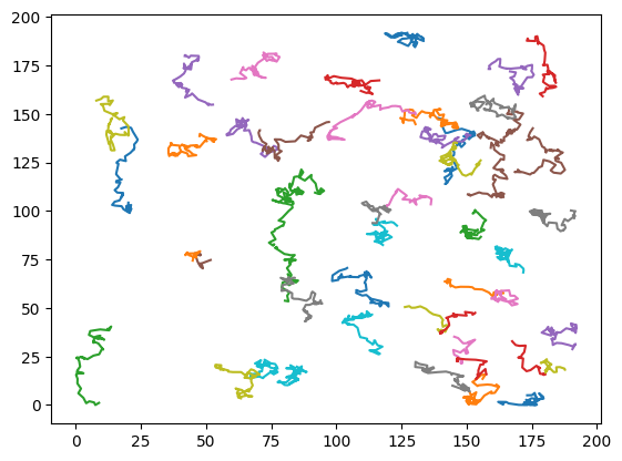
Plotting trajectories.
for traj in np.moveaxis(trajs, 0, 1): plt.plot(traj[:,0], traj[:,1])plt.show()
3. Generating videos
3.1. Import functions
For generating videos we import transform_to_video function from andi_datasets package. Additionally we import play_video function to display the videos within the jupyter notebook.
from andi_datasets.utils_videos import transform_to_video, play_video
3.2. Usage
The trajectory data generated can be directly passed through transform_to_video to generate fluorescence videos of the particles.
3.2.1. Generating a sample video
video = transform_to_video( trajs,)
play_video(video)
By default, transform_to_video function generates video like above. However, the features of the video can be easily controlled with the help of the dictionaries: particle_props, optics_props, and background_props. For detailed information about the dictionaries and the inputs they can take, please refer to the documentation of transform_to_video.
We will some example use cases of dictionaries below.
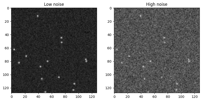
3.2.2. Controlling the noise
The noise in the videos can be controlled by adjusting the particle intensities in particle_props, and background intensity in background_props. We generate two videos in the following cell with low noise and high noise by controlling the particle intensity, for a fixed background intensity.
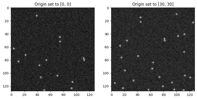
If you notice, the size of the video is always restricted to 128 x 128 px by default, while the trajectories are spread out in a larger area as per our definition of the length of the box above (Defined by simulation parameter, L). In this case, L was defined to be 1.5 * 128.
The output region of the video can be controlled in the optics_props. In the following cell, we generate the same low noise video as above but with a different region of interest (ROI). We shift the origin from [0, 0] to [30, 30], while maintaining the width and height to 128 px as before.
video_ROI = transform_to_video( trajs, particle_props={"particle_intensity": [1000, 0] }, background_props={"background_mean": 100 }, optics_props={"output_region" : [30, 30, 30+128, 30+128] # [x, y, x + width, y + height] })
fig, (ax0, ax1) = plt.subplots(ncols=2, figsize=(10, 5))ax0.imshow(low_noise_video[0], cmap="gray")ax0.set_title("Origin set to [0, 0]")ax1.imshow(video_ROI[0], cmap="gray")ax1.set_title("Origin set to [30, 30]")plt.show()
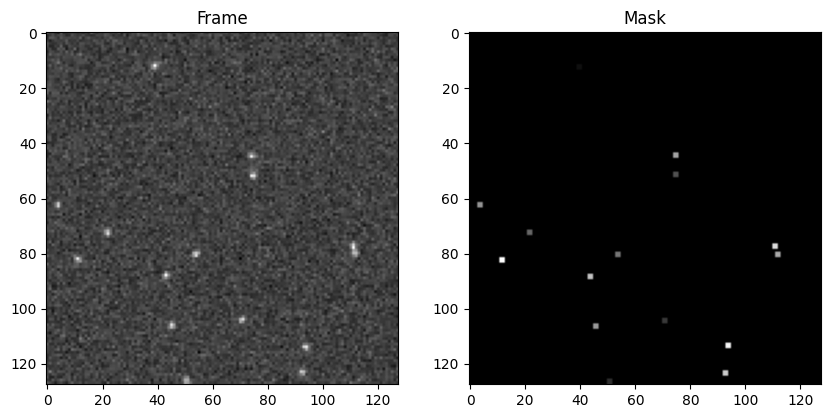
4. Generating particle masks
The transform_to_video function can generate the particle masks along with the videos.
4.1. All particle masks
By setting the parameter with_masks = True, one can generate videos and masks simultaneously. The pixel values in the masks indicate the particle numbers.
If get_vip_particles is a non-empty list, and with_masks is set to False (Default), then the output will still be a video, However, the first frame of the video now contains the masks of vip particles in the first frame.
Videos can be saved by setting save_video to True, and providing a path. Alternatively, the videos can be directly saved as numpy arrays using np.save(...).
video = transform_to_video( trajs, save_video=True, path="../Test_video.tiff")
6. Generating videos with motion blur
We can generate videos with motion blur by creating a instance of motion_blur class and passing it to transform_to_video function as a parameter.
from andi_datasets.utils_trajectories import motion_blur
Generate oversampled trajectories
output_length =50oversamp_factor =10exposure_time =0.2T = output_length * oversamp_factor # number of time steps (frames)N =50# number of particles (trajectories)L =1*128# length of the box (pixels) -> exteneding fov by 1.5 timesD =0.1# diffusion coefficient (pixels^2/frame)trajs_test, labels = models_phenom().dimerization( N=N, L=L, T=T, alphas=[1.2, 0.7], Ds=[1* D, 0.1* D], r=1, # radius of the particles Pb=1, # binding probability Pu=0, # unbinding probability)print(trajs_test.shape)
(500, 50, 2)
Initiate motion blur class with defined parameters