`models_phenom`

models_phenom

 models_phenom ()

This class handles the generation of trajectories from different theoretical models.

FBM displacements generator

source

disp_fbm

 disp_fbm (alpha:float, D:float, T:int, deltaT:int=1)

Generates normalized Fractional Gaussian noise. This means that, in general: \[ <x^2(t) > = 2Dt^{alpha} \]

and in particular: \[ <x^2(t = 1)> = 2D \]

	Type	Default	Details
alpha	float		Anomalous exponent
D	float		Diffusion coefficient
T	int		Number of displacements to generate
deltaT	int	1	Sampling time
Returns	numpy.array		Array containing T displacements of given parameters

Properties of FBM

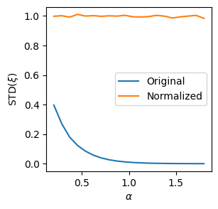
Understanding the normalization

These lines show why we need to multiply by np.sqrt(T)**alpha. Our goal is to have a random number generator with standard deviation equal to one. This does not happen with FGN above, hence the extra line:

n_disp = 10000
alphas = np.linspace(0.2, 1.8, 20)

std_og = [np.std(FGN(hurst = alpha/2).sample(n = n_disp)) for alpha in alphas]
std_norm = [np.std(FGN(hurst = alpha/2).sample(n = n_disp)*(np.sqrt(n_disp)**alpha)) for alpha in alphas]



plt.figure(figsize = (3,3))
plt.plot(alphas, std_og, label = 'Original')
plt.plot(alphas, std_norm, label = 'Normalized')                
plt.xlabel(r'$\alpha$'); plt.ylabel(r'STD($\xi$)')
plt.legend()

<matplotlib.legend.Legend>

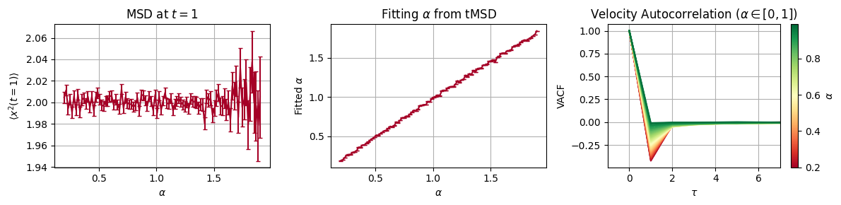
MSD and VACF

The following shows that the generated displacements have the desired properties. Namely, we can choose \(D\) and \(\alpha\) at will and the function will correctly normalize the displacements. For that, we generate trajectories and estimate parameters of the MSD and VACF from analysis class.

T = int(2e2)
alphas = np.linspace(0.2, 1.9, 100)
D = 1
reps = int(2*1e3)
tmsd_a = np.zeros((len(alphas), reps))
exp_a = np.zeros((len(alphas), 100))

taus = np.arange(0, 100)
vacf_a = np.zeros((len(alphas[alphas < 1]), len(taus)))


                  
for idx_a, alpha in enumerate(tqdm(alphas)):
    trajs = np.zeros((reps, T, 1))
    for rep in range(reps):        
        disp = models_phenom().disp_fbm(alpha, D, T, deltaT = 1)
        # Generate trajectory
        trajs[rep] = np.cumsum(disp).reshape(T, 1)
        
              
    # Calculate tMSD(tlag = 1)
    tmsd_a[idx_a] = msd_analysis().tamsd(trajs, t_lags = [1])
    exp_a[idx_a] = msd_analysis().get_exponent(trajs[:100])
    
    if alpha < 1:
        vacf_a[idx_a, :] = vacf(trajs = trajs, delta_t = 1, taus = taus)

fig, ax = plt.subplots(1, 3, figsize = (12, 3), tight_layout = True)

ax[1].errorbar(alphas, exp_a.mean(1), yerr=exp_a.std(1)/np.sqrt(reps), capsize=2, color = plt.cm.RdYlGn(0))
plt.setp(ax[1], ylabel = r'Fitted $\alpha$', xlabel = r'$\alpha$', title = r'Fitting $\alpha$ from tMSD')
ax[1].grid()

ax[0].errorbar(alphas, tmsd_a.mean(1), yerr=tmsd_a.std(1)/np.sqrt(reps), capsize=2, c = plt.cm.RdYlGn(0))
plt.setp(ax[0], ylabel = r'$\left < x^2(t=1) \right>$', xlabel = r'$\alpha$', title = r'MSD at $t=1$')
ax[0].grid()

for idxv, va in enumerate(vacf_a):
    ax[2].plot(taus, va, c = plt.cm.RdYlGn(idxv/vacf_a.shape[0]));
plt.setp(ax[2], xlim = (-1 , 7), xlabel = r'$\tau$', ylabel = 'VACF', title = r'Velocity Autocorrelation ($\alpha\in[0,1]$)')
ax[2].grid()

vec = alphas[alphas < 1]
normalize = mcolors.Normalize(vmin=vec.min(), vmax=vec.max())
colormap = plt.cm.RdYlGn
scalarmappaple = plt.cm.ScalarMappable(norm=normalize, cmap=colormap)
scalarmappaple.set_array(vec)
cbar = fig.colorbar(scalarmappaple, ax = ax[2])
cbar.set_label(r'$\alpha$')

source

_sample_diff_parameters

 _sample_diff_parameters (alphas:list, Ds:list, num_states:int,
                          epsilon_a:float, gamma_d:float)

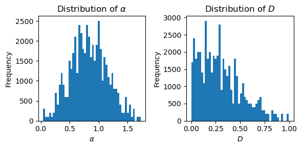
Given information of the anomalous exponents (alphas), diffusion coefficients (Ds), the function samples these from a bounded Gaussian distribution with the indicated constraints (epsilon_a, gamma_d). Outputs the list of demanded alphas and Ds.

	Type	Details
alphas	list	List containing the parameters to sample anomalous exponent in state (adapt to sampling function)
Ds	list	List containing the parameters to sample the diffusion coefficient in state (adapt to sampling function).
num_states	int	Number of diffusive states.
epsilon_a	float	Minimum distance between anomalous exponents of various states.
gamma_d	float	Factor between diffusion coefficient of various states.

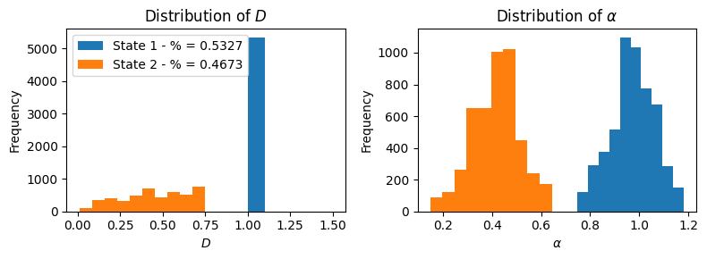
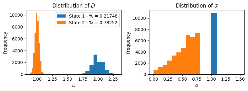
We can test that this distances are taken into account when generating trajectories:

N = 1000; L = 50; T = 2;
epsilon_a=[0.5]; gamma_d = [0.75]
trajs, labels = models_phenom().multi_state(
                                           epsilon_a=epsilon_a, gamma_d = gamma_d, # This is the important part 
                                           T = T, N = N, L = L,
                                           Ds = np.array([[2, 0], [2, 0.2]]), 
                                           alphas = np.array([[1, 0], [0.75, 0.1]]),
                                           return_state_num=True)

fig, ax = plt.subplots(1,2,figsize = (6, 3), tight_layout = True)
alphas = labels[:,:,0].flatten()
Ds = labels[:,:,1].flatten()
states_num = labels[:,:,3].flatten()
for s in np.unique(states_num):    
    ax[0].hist(alphas[states_num == s], bins = 100, density = True);
    ax[1].hist(Ds[states_num == s], bins = 100, density = True);
ax[0].set_title(fr'Distribution of $\alpha$ - $\epsilon_a = {epsilon_a[0]}$')
ax[1].set_title(fr'Distribution of $D$ - $\gamma_d = {gamma_d[0]}$')
plt.setp(ax, ylim = [0,10])
ax[0].set_xlim(0,1.1); ax[1].set_xlim(0,2.1)
ax[0].set_ylabel('Frequency')

Text(0, 0.5, 'Frequency')

Single state model

Particles diffusing according to a single diffusion state, as observed for some lipids in the plasma membrane or for nanoparticles in the cellular environment.

Single trajectory generator

source

_single_state_traj

 _single_state_traj (T:int=200, D:float=1, alpha:float=1, L:float=None,
                     deltaT:int=1, dim:int=2)

Generates a single state trajectory with given parameters.

	Type	Default	Details
T	int	200	Length of the trajectory
D	float	1	Diffusion coefficient
alpha	float	1	Anomalous exponent
L	float	None	Length of the box acting as the environment
deltaT	int	1	Sampling time
dim	int	2	Dimension of the walk (can be 2 or 3)
Returns	tuple		- pos: position of the particle - labels: anomalous exponent, D and state at each timestep. State is always free here.

Example in 2D

traj, labels = models_phenom._single_state_traj(D = 0.05,  alpha = 1.5, 
                                                T =1000, L = 10, dim = 2)

fig, ax = plt.subplots(1, 3, figsize = (10, 2), tight_layout = True)
ax[0].plot(traj[:, 0], traj[:, 1], alpha = 0.5)
plt.setp(ax[0], xlabel = 'X', ylabel = 'Y')

ax[1].plot(traj[:, 0], '.', label = 'X')
ax[1].plot(traj[:, 1], '.', label = 'Y', )
plt.setp(ax[1], ylabel = 'Position', xlabel = 'Time')
ax[1].legend()

ax[2].plot(labels[:, 0], '.', label = r'$\alpha$')
ax[2].plot(labels[:, 1], '.', label = r'$D$' )
plt.setp(ax[2], ylabel = 'Label', xlabel = 'Time')
ax[2].legend()

for b in [0,10]:
    ax[0].axhline(b, ls = '--', alpha = 0.3, c = 'k')
    ax[0].axvline(b, ls = '--', alpha = 0.3, c = 'k')
    ax[1].axhline(b, ls = '--', alpha = 0.3, c = 'k')

Example in 3D

traj, labels = models_phenom._single_state_traj(D = 0.05,  alpha = 1.5, 
                                                T =1000, L = 10, dim = 3)

fig = plt.figure(figsize = (6,5))
ax = fig.add_subplot(projection = '3d')

ax.plot(traj[:,0], traj[:,1], traj[:,2], c = 'k')
ax.scatter3D(traj[:,0], traj[:,1], traj[:,2], c = np.arange(traj.shape[0]), s = 20);
plt.setp(ax, xlabel = 'Position X', ylabel = 'Position Y', zlabel = 'Position Z',
         xticklabels = [], yticklabels = [], zticklabels = [])
ax.zaxis.labelpad=-8

Dataset generation

source

single_state

 single_state (N:int=10, T:int=200, Ds:list=[1, 0], alphas:list=[1, 0],
               L:float=None, dim:int=2)

Generates a dataset made of single state trajectories with given parameters.

	Type	Default	Details
N	int	10	Number of trajectories in the dataset
T	int	200	Length of the trajectory
Ds	list	[1, 0]	If list, mean and variance from which to sample the diffusion coefficient. If float, we consider variance = 0.
alphas	list	[1, 0]	If list, mean and variance from which to sample the anomalous exponent. If float, we consider variance = 0.
L	float	None	Length of the box acting as the environment
dim	int	2	Dimension of the walk (can be 2 or 3)
Returns	tuple		- positions: position of the N trajectories. - labels: anomalous exponent, D and state at each timestep. State is always free here.

Example in 2D

N = 500; L = 5; T = 100;
alpha = [0.8, 0.1]; D = [0.1,0.1]

trajs, labels = models_phenom().single_state(N = N,
                                           L = L,
                                           T = T, 
                                           alphas = alpha,
                                           Ds = D)
fig, ax = plt.subplots(1, 2, figsize = (6, 3), tight_layout = True)
ax[0].hist(labels[:,:,0].flatten(), bins = 50)
plt.setp(ax[0], title = r'Distribution of $\alpha$', xlabel = r'$\alpha$', ylabel = 'Frequency');

ax[1].hist(labels[:,:,1].flatten(), bins = 50)
plt.setp(ax[1], title = r'Distribution of $D$', xlabel = r'$D$', ylabel = 'Frequency');

plot_trajs(trajs, L, N)

Example in 3D

N = 4; L = 5; T = 100;
alpha = [0.8, 0.1]; D = [0.1,0.1]

trajs, labels = models_phenom().single_state(N = N,
                                           L = L,
                                           T = T, 
                                           alphas = alpha,
                                           Ds = D,
                                            dim = 3)

fig = plt.figure(figsize = (10,5))

axs = []
for idx, traj in enumerate(trajs.transpose(1,0,2)):
    ax = fig.add_subplot(1,4,idx+1, projection = '3d')

    ax.plot(traj[:,0], traj[:,1], traj[:,2], c = 'k')
    ax.scatter3D(traj[:,0], traj[:,1], traj[:,2], c = np.arange(traj.shape[0]), s = 20);
    axs.append(ax)
    
plt.setp(axs, xticklabels = [], yticklabels = [], zticklabels = []);

Multiple state model

Particles diffusing according to a time-dependent multi-state (2 or more) model of diffusion, as observed for example in proteins undergoing transient changes of \(D\) and/or \(\alpha\) as induced by, e.g., allosteric changes or ligand binding.

Single trajectory generator

source

_multiple_state_traj

 _multiple_state_traj (T=200, M=[[0.95, 0.05], [0.05, 0.95]], Ds=[1, 0.1],
                       alphas=[1, 1], L=None, deltaT=1,
                       return_state_num=False, init_state=None)

Generates a 2D multi state trajectory with given parameters.

	Type	Default	Details
T	int	200	Length of the trajectory
M	list	[[0.95, 0.05], [0.05, 0.95]]	Transition matrix between diffusive states.
Ds	list	[1, 0.1]	Diffusion coefficients of the diffusive states. Must have as many Ds as states defined by M.
alphas	list	[1, 1]	Anomalous exponents of the diffusive states. Must have as many alphas as states defined by M.
L	NoneType	None	Length of the box acting as the environment
deltaT	int	1	Sampling time
return_state_num	bool	False	If True, returns as label the number assigned to the state at each time step.
init_state	NoneType	None	If True, the particle starts in state 0. If not, sample initial state.
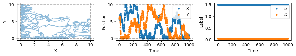
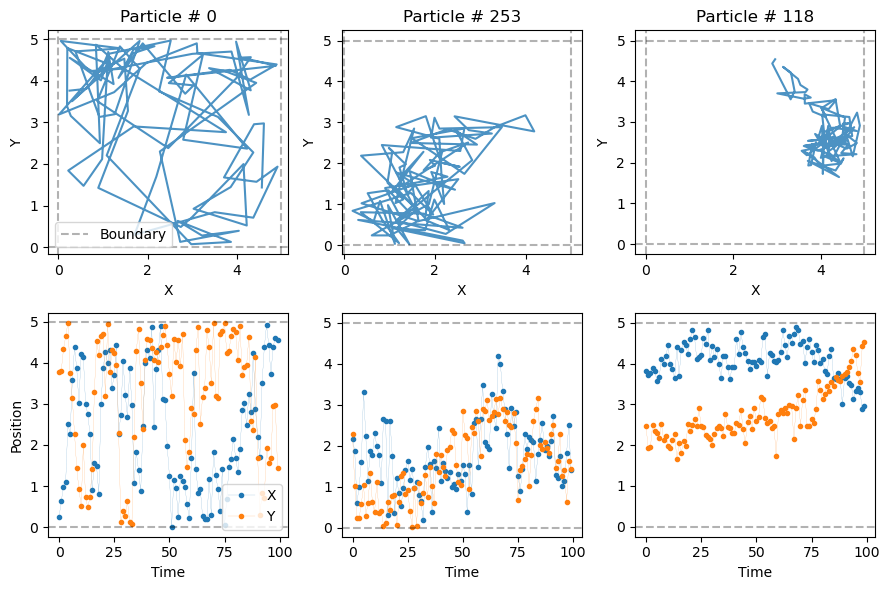
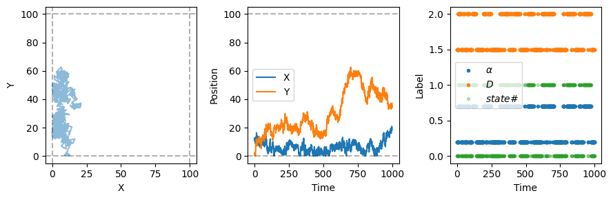
Returns	tuple		- pos: position of the particle - alphas_t: anomalous exponent at each step - Ds_t: diffusion coefficient at each step. - label_diff_state: particle’s state (can be either free or directed for alpha ~ 2) at each step. - state (optional): state label at each step.

T = 1000; L = 100
traj, labels = models_phenom._multiple_state_traj(T = T,
                                                  L = L,
                                                  alphas = [0.2, 0.7], 
                                                  Ds = [1.5, 2],                                                  
                                                  return_state_num=True)

fig, ax = plt.subplots(1, 3, figsize = (9, 3), tight_layout = True)
ax[0].plot(traj[:, 0], traj[:, 1], alpha = 0.5)
plt.setp(ax[0], xlabel = 'X', ylabel = 'Y')

ax[1].plot(traj[:, 0], label = 'X')
ax[1].plot(traj[:, 1], label = 'Y', )
plt.setp(ax[1], ylabel = 'Position', xlabel = 'Time')
ax[1].legend()

ax[2].plot(labels[:, 0], '.', label = r'$\alpha$')
ax[2].plot(labels[:, 1], '.', label = r'$D$' )
ax[2].plot(labels[:, 3], '.', label = r'$state \#$', alpha = 0.3 )
plt.setp(ax[2], ylabel = 'Label', xlabel = 'Time')
ax[2].legend()

for b in [0,L]:
    ax[0].axhline(b, ls = '--', alpha = 0.3, c = 'k')
    ax[0].axvline(b, ls = '--', alpha = 0.3, c = 'k')
    ax[1].axhline(b, ls = '--', alpha = 0.3, c = 'k')

Dataset generation

source

multi_state

 multi_state (N=10, T=200, M:<built-infunctionarray>=[[0.9, 0.1], [0.1,
              0.9]], Ds:<built-infunctionarray>=[[1, 0], [0.1, 0]],
              alphas:<built-infunctionarray>=[[1, 0], [1, 0]],
              gamma_d=None, epsilon_a=None, L=None,
              return_state_num=False, init_state=None)

Generates a dataset of 2D multi state trajectory with given parameters.

	Type	Default	Details
N	int	10	Number of trajectories
T	int	200	Length of the trajectory
M	array	[[0.9, 0.1], [0.1, 0.9]]	Transition matrix between diffusive states
Ds	array	[[1, 0], [0.1, 0]]	List of means and variances from which to sample the diffusion coefficient of each state. If element size is one, we consider variance = 0.
alphas	array	[[1, 0], [1, 0]]	List of means and variances from which to sample the anomalous exponent of each state. If element size is one, we consider variance = 0.
gamma_d	NoneType	None	Minimum factor between D of diffusive states (see ._sampling_diff_parameters)
epsilon_a	NoneType	None	Distance between alpha of diffusive states (see ._sampling_diff_parameters)
L	NoneType	None	Length of the box acting as the environment
return_state_num	bool	False	If True, returns as label the number assigned to the state at each time step.
init_state	NoneType	None	If True, the particle starts in state 0. If not, sample initial state.
Returns	tuple		- trajs (array TxNx2): particles’ position - labels (array TxNx2): particles’ labels (see ._multi_state for details on labels)

2-states

N = 100; L = 50; T = 100;

trajs, labels = models_phenom().multi_state(N = N, T = T, L = L,
                                            M = np.array([[0.95 , 0.05],[0.05, 0.95]]),
                                            Ds = np.array([[1, 0], [1, 0.5]]), 
                                            alphas = np.array([[1, 0.01], [0.5, 0.02]]),
                                            epsilon_a=[0.4], gamma_d = [0.75],
                                            return_state_num=True)

We can first check the parameter distributions:

fig, ax = plt.subplots(1, 2, figsize = (8, 3), tight_layout = True)

# Diffusion coefficients
ax[0].hist(labels[labels[:,:,3] == 0, 1].flatten(), label = f'State 1 - % = {(labels[:,:,3] == 0).sum()/np.prod(labels.shape[:2])}')
ax[0].hist(labels[labels[:,:,3] == 1, 1].flatten(), label = f'State 2 - % = {(labels[:,:,3] == 1).sum()/np.prod(labels.shape[:2])}')
plt.setp(ax[0], title = r'Distribution of $D$', xlabel = r'$D$', ylabel = 'Frequency');

# Anomalous exponents
ax[1].hist(labels[labels[:,:,3] == 0, 0].flatten(), label = f'State 1 - # = {(labels[:,:,3] == 0).sum()}')
ax[1].hist(labels[labels[:,:,3] == 1, 0].flatten(), label = f'State 2 - # = {(labels[:,:,3] == 1).sum()}')
plt.setp(ax[1], title = r'Distribution of $\alpha$', xlabel = r'$\alpha$', ylabel = 'Frequency');
ax[0].legend()

<matplotlib.legend.Legend>

And then see some examples of trajectories:

plot_trajs(trajs, L, N, labels = labels, plot_labels = True)

3-states

N = 100; L = 50; T = 100;

trajs, labels = models_phenom().multi_state(N = N, T = T, L = L,
                                            M = np.array([[0.98 , 0.01, 0.01],[0.01, 0.98, 0.01], [0.01, 0.01, 0.98]]),
                                            Ds = np.array([[1, 0], [1, 0.5], [0.1, 0]]), 
                                            alphas = np.array([[1, 0.01], [0.5, 0.02], [1.8, 0.1]]),
                                            # epsilon_a=[0.4], gamma_d = [0.75],
                                            return_state_num=True)

We can first check the parameter distributions:

fig, ax = plt.subplots(1, 2, figsize = (8, 3), tight_layout = True)

# Diffusion coefficients
ax[0].hist(labels[labels[:,:,3] == 0, 1].flatten(), label = f'State 1 - % = {(labels[:,:,3] == 0).sum()/np.prod(labels.shape[:2])}')
ax[0].hist(labels[labels[:,:,3] == 1, 1].flatten(), label = f'State 2 - % = {(labels[:,:,3] == 1).sum()/np.prod(labels.shape[:2])}')
ax[0].hist(labels[labels[:,:,3] == 2, 1].flatten(), label = f'State 3 - % = {(labels[:,:,3] == 2).sum()/np.prod(labels.shape[:2])}')
plt.setp(ax[0], title = r'Distribution of $D$', xlabel = r'$D$', ylabel = 'Frequency');

# Anomalous exponents
ax[1].hist(labels[labels[:,:,3] == 0, 0].flatten(), label = f'State 1 - # = {(labels[:,:,3] == 0).sum()}')
ax[1].hist(labels[labels[:,:,3] == 1, 0].flatten(), label = f'State 2 - # = {(labels[:,:,3] == 1).sum()}')
ax[1].hist(labels[labels[:,:,3] == 2, 0].flatten(), label = f'State 3 - # = {(labels[:,:,3] == 2).sum()}')
plt.setp(ax[1], title = r'Distribution of $\alpha$', xlabel = r'$\alpha$', ylabel = 'Frequency');
ax[0].legend()

<matplotlib.legend.Legend>

Dimerization

Particles diffusing according to a 2-state model of diffusion, with transient changes of \(D\) and/or \(\alpha\) induced by encounters with other particles, observed for example in protein dimerization.

Auxiliary functions

Distance calculator

source

_get_distance

 _get_distance (x)

Given a matrix of size Nx2, calculates the distance between the N particles.

	Type	Details
x	array	Particles’ positions
Returns	array	Distance between particles

Escaping dynamics

source

_make_escape

 _make_escape (Pu, label, diff_state)

Given an unbinding probablity (Pu), the current labeling of particles (label) and the current state of particle (diff_state, either bound, 1, or unbound, 0), simulate an stochastic binding mechanism.

	Type	Details
Pu	float	Unbinding probablity
label	array	Current labeling of the particles (i.e. to which condensate they belong)
diff_state	array	Current state of the particles
Returns	tuple	New labeling and diffusive state of the particles

Clustering dynamics

source

_make_condensates

 _make_condensates (Pb, label, diff_state, r, distance, max_label)

Given a binding probability Pb, the current label of particles (label), their current diffusive state (diff_state), the particle size (r), their distances (distance) and the label from which binding is not possible (max_label), simulates a binding mechanism.

	Type	Details
Pb	float	Binding probablity.
label	array	Current labeling of the particles (i.e. to which condensate they belong)
diff_state	array	Current state of the particles
r	float	Particle size.
distance	array	Distance between particles
max_label	int	Maximum label from which particles will not be considered for binding
Returns	tuple	New labeling and diffusive state of the particles

Here is a test in which some particles, distributed randomly through a bounded space, first bind and then unbind using the previous defined functions:

# Binding and unbinding probabilities
Pb = 0.8; Pu = 0.5
# Generate the particles
N = 200; L = 10; r = 1; max_n = 2; Ds = np.ones(100)
pos = np.random.rand(N, 2)*L    
# Put random labels (label = which condensate you belong). diff_state is zero because all are unbound)
label = np.arange(N)#np.random.choice(range(500), N, replace = False)
diff_state = np.zeros(N).astype(int)
# Define max_label bigger than max of label so everybody binds
max_label = max(label)+2
# Calculate distance between particles
distance = models_phenom._get_distance(pos)

print('# of free particles:')
print(f'Before binding: {len(label)}')

# First make particle bind:
lab, ds = models_phenom._make_condensates(Pb, label, diff_state, r, distance, max_label)
print(f'After binding: {np.unique(lab[np.argwhere(ds == 0)], return_counts=True)[0].shape[0]}')

# Then we do unbinding:
lab, ds = models_phenom._make_escape(Pu, lab, ds)
print(f'After unbinding: {np.unique(lab[np.argwhere(ds == 0)], return_counts=True)[0].shape[0]}')

# of free particles:
Before binding: 200
After binding: 4
After unbinding: 106

Stokes drag

source

_stokes

 _stokes (D)

Applies a Stokes-Einstein-like transformation to two diffusion coefficients.

	Type	Details
D	tuple	Diffusion coefficients of the two binding particles.
Returns	float	Resulting diffusion coefficient.

Time evolution

source

dimerization

 dimerization (N=10, T=200, L=100, r=1, Pu=0.1, Pb=0.01, Ds:<built-
               infunctionarray>=[[1, 0], [0.1, 0]], alphas:<built-
               infunctionarray>=[[1, 0], [1, 0]], epsilon_a=0,
               stokes=False, return_state_num=False, deltaT=1)

Generates a dataset of 2D trajectories of particles perfoming stochastic dimerization.

	Type	Default	Details
N	int	10	Number of trajectories
T	int	200	Length of the trajectory
L	int	100	Length of the box acting as the environment
r	int	1	Radius of particles.
Pu	float	0.1	Unbinding probability.
Pb	float	0.01	Binding probability.
Ds	array	[[1, 0], [0.1, 0]]	List of means and variances from which to sample the diffusion coefficient of each state. If element size is one, we consider variance = 0.
alphas	array	[[1, 0], [1, 0]]	List of means and variances from which to sample the anomalous exponent of each state. If element size is one, we consider variance = 0.
epsilon_a	int	0	Distance between alpha of diffusive states (see ._sampling_diff_parameters)
stokes	bool	False	If True, applies a Stokes-Einstein like coefficient to calculate the diffusion coefficient of dimerized particles. If False, we use as D resulting from the dimerization the D assigned to the dimerized state of one of the two particles.
return_state_num	bool	False	If True, returns as label the number assigned to the state at each time step.
deltaT	int	1	Sampling time
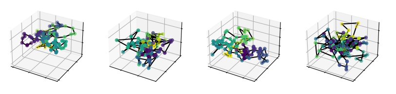
Returns	tuple		- trajs (array TxNx2): particles’ position - labels (array TxNx2): particles’ labels (see ._multi_state for details on labels)

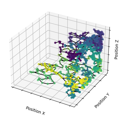
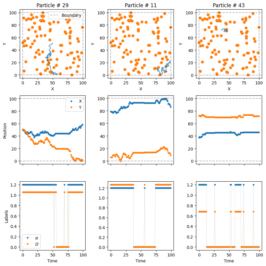
N = 500; L = 50; r = 1; T = 100
Pu = 0.1 # Unbinding probability
Pb = 1 # Binding probability
# Diffusion coefficients of two states
stokes = True
Ds = np.array([[2, 0.01], [1e-5, 0]]) # because stokes = True, we don't care about the second state
# Anomalous exponents for two states
alphas = np.array([[1, 0], [1, 0.2]]) 

trajs, labels = models_phenom().dimerization(N = N,
                                            L = L,
                                            r = r,
                                            T = T,
                                            Pu = Pu, # Unbinding probability
                                            Pb = Pb, # Binding probability
                                            Ds = Ds, # Diffusion coefficients of two states
                                            alphas = alphas, # Anomalous exponents for two states,
                                            return_state_num = True,
                                            stokes = True, epsilon_a=0.2
                                            )

fig, ax = plt.subplots(1, 2, figsize = (8, 3), tight_layout = True)

# Diffusion coefficients
ax[0].hist(labels[labels[:,:,3] == 0, 1].flatten(), label = f'State 1 - % = {(labels[:,:,3] == 0).sum()/np.prod(labels.shape[:2])}')
ax[0].hist(labels[labels[:,:,3] == 1, 1].flatten(), label = f'State 2 - % = {(labels[:,:,3] == 1).sum()/np.prod(labels.shape[:2])}')
plt.setp(ax[0], title = r'Distribution of $D$', xlabel = r'$D$', ylabel = 'Frequency');

# Anomalous exponents
ax[1].hist(labels[labels[:,:,3] == 0, 0].flatten(), label = f'State 1 - # = {(labels[:,:,3] == 0).sum()}')
ax[1].hist(labels[labels[:,:,3] == 1, 0].flatten(), label = f'State 2 - # = {(labels[:,:,3] == 1).sum()}')
plt.setp(ax[1], title = r'Distribution of $\alpha$', xlabel = r'$\alpha$', ylabel = 'Frequency');
ax[0].legend()

<matplotlib.legend.Legend>

plot_trajs(trajs, L, N, labels = labels, plot_labels = True)

Immobile traps

Particles diffusing according to a space-dependent 2-state model of diffusion, representing proteins being transiently immobilized at specific locations as induced by binding to immobile structures, such as cytoskeleton-induced molecular pinning.

source

_update_bound

 _update_bound (mask, N, pos, Nt, traps_pos, Pb, Pu, r)

Binds and unbinds particles to traps based on their position and binding and unbinding probabilities

	Type	Details
mask	array	Current binding array
N	int	Number of particles
pos	array	Position of particles
Nt	int	Number of traps
traps_pos	array	Position of traps
Pb	float in [0,1]	Binding probability
Pu	float in [0,1]	Unbinding probability
r	float	Trap radius
Returns	array	Updated binding array

source

immobile_traps

 immobile_traps (N=10, T=200, L=100, r=1, Pu=0.1, Pb=0.01, Ds=[1, 0],
                 alphas=[1, 0], Nt=10, traps_pos:<built-
                 infunctionarray>=None, deltaT=1)

Generates a dataset of 2D trajectories of particles diffusing in an environment with immobilizing traps.

	Type	Default	Details
N	int	10	Number of trajectories
T	int	200	Length of the trajectory
L	int	100	Length of the box acting as the environment
r	int	1	Radius of particles.
Pu	float	0.1	Unbinding probability.
Pb	float	0.01	Binding probability.
Ds	list	[1, 0]	Mean and variance from which to sample the diffusion coefficient of the free state. If float, we consider variance = 0
alphas	list	[1, 0]	Mean and variance from which to sample the anomalous exponent of the free state. If float, we consider variance = 0
Nt	int	10	Number of traps
traps_pos	array	None	Positions of the traps. Can be given by array or sampled randomly if None.
deltaT	int	1	Sampling time.
Returns	tuple		- trajs (array TxNx2): particles’ position - labels (array TxNx2): particles’ labels (see ._multi_state for details on labels)

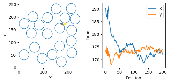
N = 50; T = 100; L = 100
# Binding and unbinding probs
Pb = 1; Pu = 0.1
# D and alpha
alpha = 1.2
D = [1, 0.2]
# Traps properties
Nt = 100
r = 1
traps_pos = np.random.rand(Nt, 2)*L 

trajs, labels = models_phenom().immobile_traps(N = N, T = T, L = L,
                                               r = r,
                                               Pu = Pu, Pb = Pb, 
                                               Ds = D, alphas = alpha,
                                               Nt = Nt, traps_pos = traps_pos
                                              )

plot_trajs(trajs, L, N, labels = labels, plot_labels = True, traps_positions=traps_pos)

Confinement

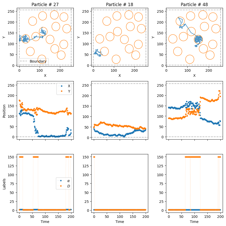
Particles diffusing according to a space-dependent 2-state model of diffusion, observed for example in proteins being transiently confined in regions where diffusion properties might change, e.g., the confinement induced by clathrin-coated pits on the cell membrane. In the limit of a high density of trapping regions, this model reproduces the picket-and-fence model used to describe the effect of the actin cytoskeleton on transmembrane proteins.

Auxiliary functions

Distribute compartments

source

_distribute_circular_compartments

 _distribute_circular_compartments (Nc, r, L)

Distributes circular compartments over an environment without overlapping. Raises a warning and stops when no more compartments can be inserted.

	Type	Details
Nc	float	Number of compartments
r	float	Size of the compartments
L	float	Side length of the squared environment.
Returns	array	Position of the centers of the compartments

fig, ax = plt.subplots(figsize = (5,5))

Nc = 60; r = 10; L = 256;
comp_center = models_phenom._distribute_circular_compartments(Nc, r, L)

for c in comp_center:
    circle = plt.Circle((c[0], c[1]), r)
    ax.add_patch(circle)
ax.set_xlim(0,L)
ax.set_ylim(0,L)

(0.0, 256.0)

Reflection inside circles

source

_reflected_position

 _reflected_position (circle_center, circle_radius, beg, end,
                      precision_boundary=0.0001)

Given the begining and end of a segment crossing the boundary of a circle, calculates the new position considering that boundaries are fully reflective.

	Type	Default	Details
circle_center	float		Center of the circle
circle_radius	float		Radius of the circle
beg	tuple		Position (in 2D) of the begining of the segment
end	tuple		Position (in 2D) of the begining of the segment
precision_boundary	float	0.0001	Small area around the real boundary which is also considered as boundary. For numerical stability
Returns	tuple		- Reflected position - Intersection point

circle_radius = 2;
circle_center = [0,0]
beg = np.array([0.8, 0])+circle_center
end = np.array([2.5, -0.8])+circle_center

final_point, intersect = models_phenom._reflected_position(circle_center, circle_radius, beg, end)

fig, ax = plt.subplots(figsize = (3, 3))

circle = plt.Circle(circle_center, circle_radius, facecolor = 'w', ec = 'C0', label = 'Compartment', zorder = -1)
ax.add_patch(circle)
ax.plot([beg[0],end[0]], [beg[1], end[1]], '-o', c = 'C1', label = 'Displacement segment')
ax.plot([circle_center[0], intersect[0]], [circle_center[1], intersect[1]], c = 'C2')
ax.plot([intersect[0], final_point[0]], [intersect[1], final_point[1]], '-o', c = 'C4', label = 'Resulting reflection')
ax.set_ylim(circle_center[1]-circle_radius*1.5, circle_center[1]+circle_radius*1.5)
ax.set_xlim(circle_center[0]-circle_radius*1.5, circle_center[0]+circle_radius*1.5)
ax.legend(fontsize = 8)

<matplotlib.legend.Legend>

Single trajectory generator

source

_confinement_traj

 _confinement_traj (T=200, L=100, Ds=[1, 0.1], alphas=[1, 1], r=1,
                    comp_center=None, Nc=10, trans=0.1, deltaT=1)

Generates a 2D trajectory of particles diffusing in an environment with partially transmitting circular compartments.

	Type	Default	Details
T	int	200	Length of the trajectory
L	int	100	Length of the box acting as the environment
Ds	list	[1, 0.1]	Diffusion coefficients of the two diffusive states (first free, the confined). Size must be 2.
alphas	list	[1, 1]	Anomalous exponents of the two diffusive states (first free, the confined). Size must be 2.
r	int	1	Radius of the compartments.
comp_center	NoneType	None	If given, center of the compartments. If None, centers are uniformly sampled.
Nc	int	10	Number of compartments
trans	float	0.1	Transmittance of the boundaries
deltaT	int	1	Sampling time.
Returns	tuple		- pos (array Tx2): particle’s position - labels (array Tx2): particle’s labels (see ._multi_state for details on labels)

N = 50;  L = 20
Nc = 15; r = 1; L = 20
Ds = [1, 0.1]
r , L, Nc = (20, 256, 20)

comp_center = models_phenom._distribute_circular_compartments(Nc = Nc, r = r, L = L)
trajs, labels = models_phenom()._confinement_traj(trans = 0.1, Nc = Nc, r = r, L = L, T =200, comp_center=comp_center, Ds = Ds)

fig, axs = plt.subplots(1,2, figsize = (6,3), tight_layout = True)

ax = axs[0]
for c in comp_center:
    circle = plt.Circle((c[0], c[1]), r, facecolor = 'None', edgecolor = 'C0')
    ax.add_patch(circle)    
ax.scatter(trajs[:,0], trajs[:,1], c = plt.cm.cividis(labels[:,-1]/2), zorder = -1, s = 2)   

plt.setp(axs[0], xlim = (0,L), ylim = (0,L), xlabel = 'X', ylabel = 'Y')

axs[1].plot(trajs[:,0], label = 'x');
axs[1].plot(trajs[:,1], label = 'y');
axs[1].legend()
plt.setp(axs[1], xlabel = 'Position', ylabel = 'Time')

[Text(0.5, 0, 'Position'), Text(0, 0.5, 'Time')]

Dataset generation

source

confinement

 confinement (N=10, T=200, L=100, Ds=[[1, 0], [0.1, 0]], alphas=[[1, 0],
              [1, 0]], gamma_d=[1], epsilon_a=[0], r=1, comp_center=None,
              Nc=10, trans=0.1, deltaT=1)

Generates a dataset of 2D trajectories of particles diffusing in an environment with partially transmitting circular compartments.

	Type	Default	Details
N	int	10	Number of trajectories
T	int	200	Length of the trajectory
L	int	100	Length of the box acting as the environment
Ds	list	[[1, 0], [0.1, 0]]	List of means and variances from which to sample the diffusion coefficient of each state. If element size is one, we consider variance = 0.
alphas	list	[[1, 0], [1, 0]]	List of means and variances from which to sample the anomalous exponent of each state. If element size is one, we consider variance = 0.
gamma_d	list	[1]	Minimum factor between D of diffusive states (see ._sampling_diff_parameters). Size is number of states -1 (in this case size 1)
epsilon_a	list	[0]	Distance between alpha of diffusive states (see ._sampling_diff_parameters). Size is number of states -1 (in this case size 1)
r	int	1	Radius of the compartments.
comp_center	NoneType	None	If given, center of the compartments. If None, centers are uniformly sampled.
Nc	int	10	Number of compartments
trans	float	0.1	Transmittance of the boundaries
deltaT	int	1	Sampling time.
Returns	tuple		- pos (array Tx2): particle’s position - labels (array Tx2): particle’s labels (see ._multi_state for details on labels)

N = 50;  L = 20
Nc = 15; r = 1; L = 20
Ds = [[1,0], [150,0.1]]
alphas = [[1, 0], [1.5,0.1]]
r , L, Nc = (20, 256, 15)
comp_center = models_phenom._distribute_circular_compartments(Nc = Nc, r = r, L = L)
trajs, labels = models_phenom().confinement(N = N, L = L, comp_center = comp_center, trans = 0.1, Ds = Ds, 
                                            r = r, alphas = alphas, epsilon_a = [0])

plot_trajs(trajs, L, N, labels = labels, plot_labels = True, comp_center = comp_center, r_cercle=r)