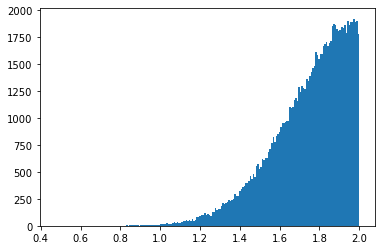
utils_trajectories

Probability distributions

Pert distribution

---

source

pert

 pert (params:list, size:int=1, lamb=4)

Samples from a Pert distribution of given parameters

	Type	Default	Details
params	list		Pert parameters a, b, c
size	int	1	number of samples to get
lamb	int	4	lambda pert parameters
Returns	array		samples from the given Pert distribution

Gaussian distribution

---

source

gaussian

 gaussian (params:list|int, size=1, bound=None)

Samples from a Gaussian distribution of given parameters.

	Type	Default	Details
params	list | int		If list, mu and sigma^2 of the gaussian. If int, we consider sigma = 0
size	int	1	Number of samples to get.
bound	NoneType	None	Bound of the Gaussian, if any.
Returns	array		Samples from the given Gaussian distribution

k = gaussian([2, 0.1], size = int(1e5), bound = [0, 2])
plt.hist(k, bins = 200);

Sampler random points in the surface of a sphere

---

source

sample_sphere

 sample_sphere (N:int, R:int|list)

Samples random number that lay in the surface of a 3D sphere centered in zero and with radius R.

	Type	Details
N	int	Number of points to generate.
R	int | list	Radius of the sphere. If int, all points have the same radius, if numpy.array, each number has different radius.
Returns	array	Sampled numbers

1D Brownian motion

---

source

bm1D

 bm1D (T:int, D:float, deltaT=False)

Creates a 1D Brownian motion trajectory

	Type	Default	Details
T	int		Length of the trajecgory
D	float		Diffusion coefficient
deltaT	bool	False	Sampling time
Returns	array		Brownian motion trajectory

Regularize and normalize

Regularize trajectory with irregular sampling times

---

source

regularize

 regularize (positions:<built-infunctionarray>, times:<built-
             infunctionarray>, T:int)

Regularizes a trajectory with irregular sampling times.

	Type	Details
positions	array	Positions of the trajectory to regularize
times	array	Times at which previous positions were recorded
T	int	Length of the output trajectory
Returns	array	Regularized trajectory.

Normalize displacements of a trajectory

---

source

normalize

 normalize (trajs)

Normalizes trajectories by substracting average and dividing by SQRT of their standard deviation.

	Type	Details
trajs	np.array	Array of length N x T or just T containing the ensemble or single trajectory to normalize.

---

source

normalize_fGN

 normalize_fGN (disp, alpha, D, T:int, deltaT:int=1)

Normalizes fractional Gaussian Noise created with stochastic library.

	Type	Default	Details
disp	Array-like of shape N x T or just T containing the displacements to normalize.
alpha	float in [0,2] or array-like of length N x 1		Anomalous exponent
D	float or array-like of shape N x 1		Diffusion coefficient
T	int		Number of timesteps the displacements were generated with
deltaT	int	1	Sampling time
Returns	Array-like containing T displacements of given parameters

N = 10; T = 10
trajs = 3*np.random.randn(N*T*2).reshape(N,T,2)
trajs = np.cumsum(trajs, axis = 1)

norm_trajs = normalize(trajs)

idx = 0; plt.figure(figsize = (3,3))
plt.plot(trajs[idx,:,0]-trajs[idx,0,0], '-o', label = 'Original trajectory')
plt.plot(norm_trajs[idx,:,0], '-o', label = 'Normalized')
plt.legend(); plt.xlabel('Time'); plt.ylabel('Position')

Text(0, 0.5, 'Position')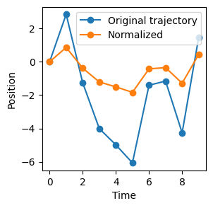

Trigonometry functions

Needed for the correct calculation of confined diffusion in circular compartments.

---

source

trigo

 trigo ()

This class gathers multiple useful trigonometric relations.

Inspired from: https://stackoverflow.com/questions/30844482/what-is-most-efficient-way-to-find-the-intersection-of-a-line-and-a-circle-in-py and http://mathworld.wolfram.com/Circle-LineIntersection.html

---

source

trigo.circle_line_segment_intersection

 trigo.circle_line_segment_intersection (circle_center, circle_radius,
                                         pt1, pt2, full_line=False,
                                         tangent_tol=1e-09)

Find the points at which a circle intersects a line-segment. This can happen at 0, 1, or 2 points.

	Type	Default	Details
circle_center	tuple		The (x, y) location of the circle center
circle_radius	float		The radius of the circle
pt1	tuple		The (x, y) location of the first point of the segment
pt2	tuple		The (x, y) location of the second point of the segment
full_line	bool	False	True to find intersections along full line - not just in the segment. False will just return intersections within the segment.
tangent_tol	float	1e-09	Numerical tolerance at which we decide the intersections are close enough to consider it a tangent
Returns	Sequence[Tuple[float, float]]		A list of length 0, 1, or 2, where each element is a point at which the circle intercepts a line segment.

Adding field of view (FOV)

---

source

find_nan_segments

 find_nan_segments (a, cutoff_length)

Extract all segments of nans bigger than the set cutoff_length. If no segments are found, returns None. For each segments, returns the begining and end index of it.

Output: array of size (number of segments) x 2.

---

source

segs_inside_fov

 segs_inside_fov (traj, fov_origin, fov_length, cutoff_length)

Given a trajectory, finds the segments inside the field of view (FOV).

	Type	Details
traj	array	Set of trajectories of size N x T (N: number trajectories, T: length).
fov_origin	tuple	Bottom right point of the square defining the FOV.
fov_length	float	Size of the box defining the FOV.
cutoff_length	float	Minimum length of a trajectory inside the FOV to be considered in the output dataset.
Returns	array	Set of segments inside the FOV.

---

source

inside_fov_dataset

 inside_fov_dataset (trajs, labels, fov_origin, fov_length,
                     cutoff_length=10, func_labels=None,
                     return_frames=False)

Given a dataset of trajectories with labels and a FOV parameters, returns a list of trajectories with the corresponding labels inside the FOV

	Type	Default	Details
trajs	array		Set of trajectories with shape T x N x 2.
labels	array		Set of labels with shape T x N x 2.
fov_origin	tuple		Bottom left point of the square defining the FOV.
fov_length	float		Size of the box defining the FOV.
cutoff_length	int	10	Minimum length of a trajectory inside the FOV to be considered in the output dataset.
func_labels	NoneType	None	(optional) Function to be applied to the labels to take advantage of the loop.
return_frames	bool	False
Returns	tuple		- trajs_fov (list): list 2D arrays containing the trajectories inside the field of view. - labels_fov (list): corresponding labels of the trajectories.

Example: (check notebooks for full details)

L = 200; T = 100
Ns = [20,10,10]
alphas = [1,1.5]
D = 1   

trajs, labels = models_phenom().multi_state(N = 500, L = L, T = 50)

fov_origin = [50,50]; fov_length = L*0.1
trajs_fov, labels_fov = inside_fov_dataset(trajs, labels, fov_origin, fov_length)

fig, (ax, ax2) = plt.subplots(1, 2, figsize = (14,7))
colors = plt.cm.RdYlGn(np.linspace(0, 1, len(trajs_fov)))

for idx, og_traj in enumerate(trajs[:, :, :].transpose(1,0,2)):
    ax.plot(og_traj[:, 0], og_traj[:, 1], c = 'k', alpha = 0.5, lw = 0.8)

for t, c in zip(trajs_fov, colors[::-1, :]):
    ax.plot(t[0], t[1], c= c)
    ax2.scatter(t[0], t[1], facecolor = c, s = 1)

# FOV
fov_min_x, fov_min_y = fov_origin
fov_max_x, fov_max_y = np.array(fov_origin)+fov_length
# currentAxis = ax.gca()
ax.add_patch(Rectangle((fov_min_x, fov_min_y), fov_length, fov_length, fill=None, alpha=1, lw = 2, label = 'FOV'))


# Boundary
ax.axhline(0,  alpha = 0.5, ls = '--', c = 'k', label = 'boundary')
ax.axhline(L,  alpha = 0.5, ls = '--', c = 'k')
ax.axvline(0,  alpha = 0.5, ls = '--', c = 'k')
ax.axvline(L,  alpha = 0.5, ls = '--', c = 'k')

# FOV origin
ax.scatter(fov_origin[0], fov_origin[1], label = 'FOV origin', s = 40, zorder = 10)

legend = ax.legend()
legend.get_frame().set_alpha(None)
plt.setp(ax, xlabel = 'X (px)', ylabel = 'Y (px)')
plt.setp(ax2, xlim = (0,L), ylim = (0,L));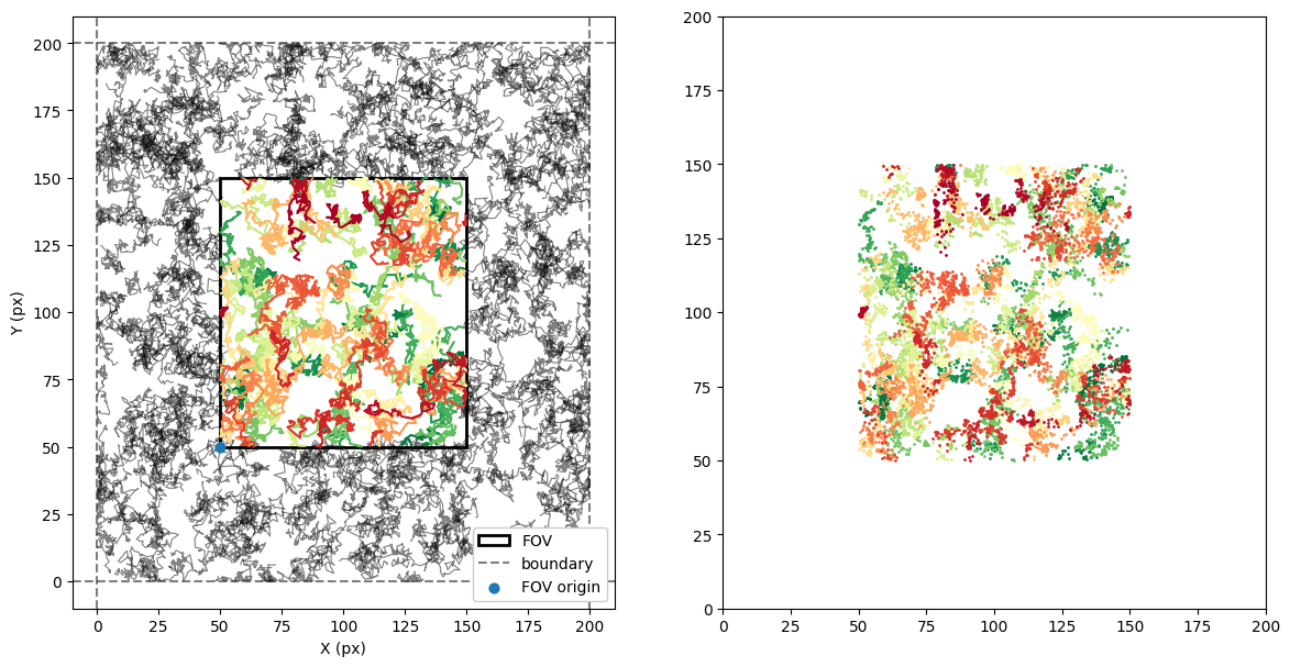

Motion Blur

---

source

motion_blur

 motion_blur (output_length:int, oversamp_factor:float=10,
              exposure_time:float=0.5)

Applies a motion blur to given trajectories. Motion blur is apply by considering an oversampled trajectory and then averaging the position over the exposure time. The oversampling is controled by the oversampling factor O.

If we want to generate trajectories of size T, we must input trajectories of size T*O. The trajectory is then reshape into chunks of size O. The output position for each chunk is the average over the exposure time, i.e. the percentage of the beginning of this chunk.

	Type	Default	Details
output_length	int		Expected length of trajectories after applying motion blur
oversamp_factor	float	10	Oversampling factor. This implies that the number of frames goes from input -> T*O to output -> T
exposure_time	float	0.5	Percentage of the oversampled (i.e in [0,1])

---

source

motion_blur.apply

 motion_blur.apply (trajs:<built-infunctionarray>)

Applies the motion blur with the parameters defined.

	Type	Details
trajs	array	Input trajectories. Must be of size (input_length, num_trajs, dimension)
Returns	array	Output trajectories after applying motion blur. Size: (input_length / oversamp_factor, num_trajs, dimension)

Example:

MB = motion_blur(output_length = 10, oversamp_factor = 10, exposure_time = 0.5)
trajs = np.random.randn(100, 5, 2).cumsum(0)
trajs[:,0,0] = np.arange(100) # we put a straight line to check what happens
mb_trajs = MB.apply(trajs)

_, axs = plt.subplots(2,5,figsize = (15,6))

for t, t_mb, ax in zip(trajs.transpose(1,0,2), mb_trajs.transpose(1,0,2), axs.transpose()):
    
    ax[0].plot(np.linspace(0,10,t.shape[0]), t[:,0], label = 'OG traj')
    ax[0].plot(np.linspace(0,10,t_mb.shape[0]), t_mb[:,0], 'o-', alpha = 0.8, label = 'motion blur')
    
    ax[1].plot(np.linspace(0,10,t.shape[0]), t[:,1])
    ax[1].plot(np.linspace(0,10,t_mb.shape[0]), t_mb[:,1], 'o-', alpha = 0.8)
axs[0,0].legend()
plt.setp(axs, yticklabels = []);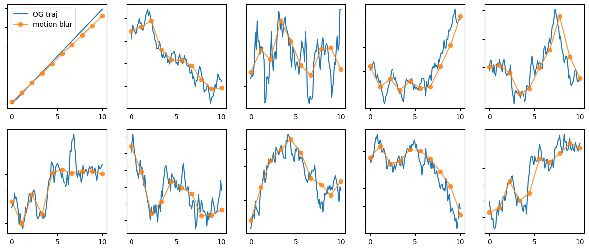

Plotting trajectories

---

source

plot_trajs

 plot_trajs (trajs, L, N, num_to_plot=3, labels=None, plot_labels=False,
             traps_positions=None, traps_r=None, comp_center=None,
             r_cercle=None)

T = 50; N = 50; L = 1.2*128; D = 0.1

trajs_model1, labels = models_phenom().single_state(N = N, 
                                            L = L,
                                            T = T,
                                            Ds = D,
                                            alphas = 0.5
                                            )

plot_trajs(trajs_model1, L, N)