analysis

Angle calculation

---

source

dataset_angles

 dataset_angles (trajs:list)

Given a set of trajectories, calculate all angles between displacements

	Type	Details
trajs	list	set of trajectories from which to calculate angles
Returns	list	list of angles between displacements

---

source

get_angle

 get_angle (a:tuple, b:tuple, c:tuple)

Calculates the angle between the segments generate by three points

	Type	Details
a	tuple	2d position point A
b	tuple	2d position point B
c	tuple	2d position point C
Returns	tuple	angle between segments AB and BC points

MSD based analysis

---

source

msd_analysis

 msd_analysis ()

Contains mean squared displacement (MSD) based methods to analyze trajectories.

---

source

msd_analysis.tamsd

 msd_analysis.tamsd (trajs:numpy.ndarray, t_lags:numpy.ndarray, dim=1)

Calculates the time average mean squared displacement (TA-MSD) of a trajectory at various time lags,

	Type	Default	Details
trajs	ndarray		Set of trajectories of dimenions NxTxD (N: number of trajectories, T: lenght, D: dimension)
t_lags	ndarray		Time lags used for the TA-MSD
dim	int	1	Dimension of the trajectories (currently only 1 and 2 supported)
Returns	np.array		TA-MSD of each trayectory / t_lag

---

source

msd_analysis.get_diff_coeff

 msd_analysis.get_diff_coeff (trajs:numpy.ndarray, t_lags:list=None)

Calculates the diffusion coefficient of a trajectory by means of the linear fitting of the TA-MSD.

	Type	Default	Details
trajs	ndarray
t_lags	list	None	Time lags used for the TA-MSD.
Returns	np.array		Diffusion coefficient of the given trajectory.

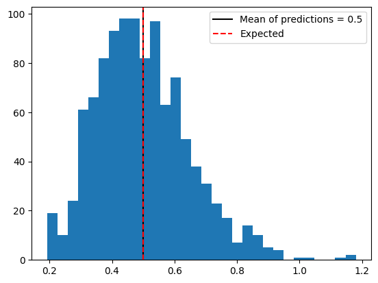
Here we show an example for the calculation of the diffusion coefficient of a 2D Brownian motion trajectory. We create trajectories from displacements of variance \(\sigma =1\), which results in a diffusion coefficient \(D=0.5\).

pos = np.cumsum(np.random.randn(1070, 100, 2), axis = 1)
D = msd_analysis().get_diff_coeff(pos)

plt.hist(D, bins = 30);
plt.axvline(np.mean(D), c = 'k', label = f'Mean of predictions = {np.round(np.mean(D), 2)}')                                                                  
plt.axvline(0.5, c = 'r', ls = '--', label = 'Expected')
plt.legend()

<matplotlib.legend.Legend>

---

source

msd_analysis.get_exponent

 msd_analysis.get_exponent (trajs:numpy.ndarray, t_lags:list=None)

Calculates the diffusion coefficient of a trajectory by means of the linear fitting of the TA-MSD.

	Type	Default	Details
trajs	ndarray
t_lags	list	None	Time lags used for the TA-MSD.
Returns	np.array		Diffusion coefficient of the given trajectory.

To showcase this function, we generate fractional brownian motion trajectories with \(\alpha = 0.5\) and calculate their exponent:

trajs, _ = models_phenom().single_state(N = 1001, T = 100, alphas = 0.5, dim = 2)
alpha = msd_analysis().get_exponent(trajs.transpose(1,0,2))

plt.hist(alpha, bins = 30);
plt.axvline(np.mean(alpha), c = 'k', label = f'Mean of predictions = {np.round(np.mean(alpha), 2)}')
plt.axvline(0.5, c = 'r', ls = '--', label = 'Expected')
plt.legend()

(1001, 100, 2)

<matplotlib.legend.Legend>

Velocity Autocorrelation Function (VACF)

---

source

vacf

 vacf (trajs, delta_t:int|list|numpy.ndarray=1,
       taus:bool|list|numpy.ndarray=None)

Calculates the velocity autocorrelation function for the given set of trajectories.

	Type	Default	Details
trajs	np.array		NxT matrix containing N trajectories of length T.
delta_t	int | list | numpy.ndarray	1	If not None, the vacf is calculated in the demanded time lags.
taus	bool | list | numpy.ndarray	None	Time windows at wich the vacf is calculated.
Returns	np.array		VACF of the given trajectories and the given time windows.

We show here an example of the VACF for FBM trajectories at various time lages, showing that they all coincide (as expected for this diffusion model).

deltats = np.arange(1, 5).tolist()
taus = np.arange(0, 100)
trajs, _ = models_phenom().single_state(N = 200, T = 200, alphas = 0.5)
trajs = trajs.transpose(1, 0, 2)[:,:,0]

for deltat in deltats:  
    v = vacf(trajs, deltat, taus)        
    plt.plot(taus/deltat, v.flatten(), 'o-', alpha = 0.4)    
plt.xlim(-1, 10)
plt.ylabel('VACF'); plt.xlabel(r'$\tau / \delta$')

Text(0.5, 0, '$\\tau / \\delta$')

Convex hull analysis

---

source

CH_changepoints

 CH_changepoints (trajs, tau:int=10, metric:{'volume','area'}='volume')

Computes the changes points a multistate trajectory based on the Convex Hull approach proposed in PRE 96 (022144), 2017.

	Type	Default	Details
trajs	np.array		NxT matrix containing N trajectories of length T.
tau	int	10	Time window over which the CH is calculated.
metric	{‘volume’, ‘area’}	volume	Calculate change points w.r.t. area or volume of CH.
Returns	list		Change points of the given trajectory.

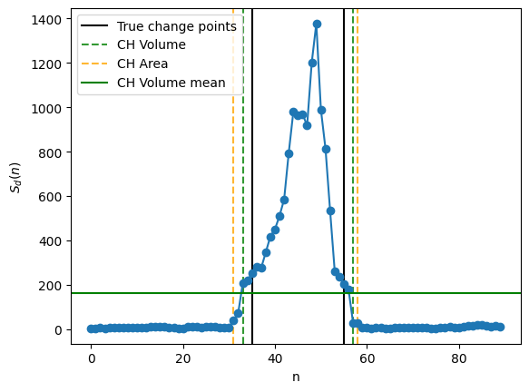
We showcase the use of the convex hull in a Brownian motion trajectory with two distinct diffusion coefficients, one 10 times the other:

# Generate trajectories and plot change points
T = 100; on = 40; off = 60; tau = 5
traj = np.random.randn(T, 2)
traj[on:off, :] = traj[on:off, :]*10
traj = traj.cumsum(0)
plt.axvline(on-tau, c = 'k')
plt.axvline(off-tau, c = 'k', label = 'True change points')

# Calculate variable Sd 
Sd = np.zeros(traj.shape[0]-2*tau)
for k in range(traj.shape[0]-2*tau):       
    Sd[k] = ConvexHull(traj[k:(k+2*tau)], ).volume  

# Compute change points both with volume and area
CPs = CH_changepoints([traj], tau = tau)[0].flatten()-tau
CPs_a = CH_changepoints([traj], tau = tau, metric = 'area')[0].flatten()-tau


# Plot everything
label_cp = 'CH Volume'
for cp in CPs:
    plt.axvline(cp, c = 'g', alpha = 0.8, ls = '--', label = label_cp)
    label_cp = ''
label_cp = 'CH Area'    
for cp in CPs_a:
    plt.axvline(cp, alpha = 0.8, ls = '--', c = 'orange', label = label_cp)
    label_cp = ''
    
plt.plot(Sd, '-o')
plt.axhline(Sd.mean(), label = 'CH Volume mean', c = 'g',)
plt.legend()
plt.xlabel('n'); plt.ylabel(r'$S_d(n)$')

Text(0, 0.5, '$S_d(n)$')

Cramér-Rao lower bound

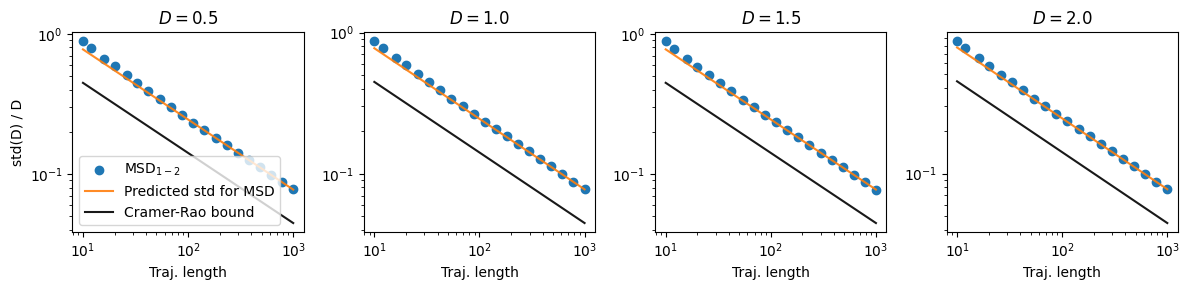
Expressions of the CRLB for the estimation of the diffusion coefficient for trajectories without noise, for dimension 1 and 2, at different trajectory lengths

---

source

CRLB_D

 CRLB_D (T:int, dim:int=1)

Returns the Cramer-Rao lower bound S(D)/D for Brownian motion without noise, namely

S(D) / D = sqrt(2 / (d·T) )

	Type	Default	Details
T	int		Length of the trajectory
dim	int	1	Dimension of the trajectoy
Returns	float		Cramér-Rao bound

Here we show how for Brownian motion trajectories, the MSD with is nearly optimal and follows the same scaling as the CRLB (i.e. \(S(D)/D = \sqrt(6/T)\).

Ts = np.logspace(1, 3,20).astype(int) # Trajectory lengths
Ds = np.arange(0.5, 2.1, 0.5) # We will test on different diffusion coefficients

# Saving the standard deviations
std_ds = np.zeros((len(Ds), len(Ts)))

for idxD, D in enumerate(tqdm(Ds)):
    
    # Generate the BM trajectories with given parameters
    trajs = (np.sqrt(2*D)*np.random.randn(int(1e4), Ts[-1], 1)).cumsum(1) 

    for idxL, T in enumerate(tqdm(Ts)):
        
        std_ds[idxD, idxL] = np.array(msd_analysis().get_diff_coeff(trajs = trajs[:, :T], t_lags = [1,2])).std()

fig, axs = plt.subplots(1,4, figsize = (4*3,3), tight_layout = True)

for idx, (ax, std_d, D) in enumerate(zip(axs.flatten(), std_ds, Ds)):
    ax.scatter(Ts, std_d/D, label = r'MSD$_{1-2}$')
    ax.loglog(Ts, np.sqrt(6/Ts), label = 'Predicted std for MSD', alpha = 0.9, c = 'C1')
    ax.loglog(Ts, CRLB_D(Ts), label = 'Cramer-Rao bound', alpha = 0.9, c = 'k')
    ax.set_title(fr'$D = {D}$')
axs[0].legend()
plt.setp(axs[0], ylabel = 'std(D) / D')
plt.setp(axs, xlabel = 'Traj. length');

Bounds for \(\alpha\) and \(K_{alpha}\) in FBM

---

source

derivative_covariance_matrix_K_alpha

 derivative_covariance_matrix_K_alpha (alpha, K_alpha, N, delta_t=1.0)

Calculate the derivative of the covariance matrix with respect to K_alpha.

---

source

derivative_covariance_matrix_alpha

 derivative_covariance_matrix_alpha (alpha, K_alpha, N, delta_t=1.0)

Calculate the derivative of the covariance matrix with respect to alpha using vectorized operations.

---

source

generate_covariance_matrix

 generate_covariance_matrix (alpha, K_alpha, N, delta_t=1.0)

Generate the covariance matrix for FBM using vectorized operations.

---

source

fisher_information_matrix

 fisher_information_matrix (alpha, K_alpha, N, delta_t=1.0)

Calculate the full Fisher Information Matrix and its inverse.

---

source

fisher_information_cross

 fisher_information_cross (alpha, K_alpha, N, delta_t=1.0)

Calculate the Fisher Information cross term I_alpha,K_alpha.

---

source

fisher_information_K_alpha

 fisher_information_K_alpha (K_alpha, N, delta_t=1.0)

Calculate the Fisher Information component I_K_alpha,K_alpha.

In this case, it can be analytically calculate as N/(2*K_alpha**2)

---

source

fisher_information_alpha

 fisher_information_alpha (alpha, N, delta_t=1.0)

Calculate the Fisher Information component I_alpha,alpha.

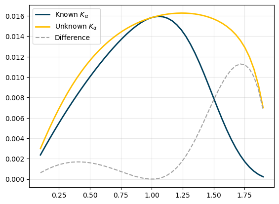
Example: CRLB of \(\alpha\) for unknown and known \(K_\alpha\)

# Example parameters
alphas = np.linspace(0.1, 1.9, 50) # anomalous exponent to check
T = 100  # Length of the trajectory
K_alpha = 1 # diffusion coefficient (note that these results are independnet of K_alpha)

# Variance with known K_alpha (i.e. inverse of diagonal term of the Fisher information matrix)
var_a_k = np.array([1/fisher_information_alpha(alpha, T) for alpha in alphas])

# Variance with unknown K_alpha (i.e. diagonal term of the inverse of the full Fisher information matrix)
var_a_uk = np.array([fisher_information_matrix(alpha, K_alpha, T)[1][0,0] for alpha in alphas])


plt.plot(alphas, var_a_k, c = '#003f5c', lw = 2, label = r'Known $K_\alpha$')
plt.plot(alphas, var_a_uk, c = '#ffbf00', lw = 2, label = r'Unknown $K_\alpha$')
plt.plot(alphas, var_a_uk-var_a_k, c = '#a3a3a3', ls = '--', label = 'Difference')
plt.grid(alpha = 0.3)
plt.xlabel(r'$\alpha$')
plt.legend()

<matplotlib.legend.Legend>

p-variation

---

source

p_variation

 p_variation (traj:<built-infunctionarray>, m:int, p:int)

Given a trajectory, computes the p-variation for the given lag m and variation p.

	Type	Details
traj	array	Trajectory for which to compute the p-variation
m	int	Time lag between positions considered in the p-variation (see Eq. (8) of https://doi.org/10.1103/PhysRevE.82.021130)
p	int	Integer defining the p-variation
Returns	array	p-variation of the current trajectory

---

source

p_variation_FBM

 p_variation_FBM (H:float, sigma:float, t:<built-infunctionarray>)

Given a Hurst exponent and the std of a FBM process with MSD = sigma^2 t^(2H), computes the predicted p-variation:

p^(1/H) (t) = E(|B(1)|^(1/H))

See more at Eq. (8) in https://doi.org/10.1103/PhysRevE.82.011129

	Type	Details
H	float	Hurst exponent
sigma	float	Standard deviation of the FBM process
t	array	times for which to compute p^(1/H) (t)
Returns	array	Theoretical prediction for the p^(1/H) (t)

Example 1: p-variation scaling for p = 2

In the case of p = 2, based on [1]:

• For FBM: we should have an increasing p-variation with bigger resolution (in the paper it means increasing n in Eq.(5) but in the discrete version used here it means decreasing m (see Eq. (8) of [2]).
• For CTRW: the p-variation should estabilize to a value given [1] (i.e smaller m should start converging to this stable value).

T = 5000
H = 0.2

fbm_traj = models_theory().fbm(alpha = H*2, T = T)
ctrw_traj = models_theory().ctrw(alpha = H*2, T = T)

fig, ax = plt.subplots(1, 2, figsize = (7,3))

for m in [1,2,3,4,5]:
   
    pvar_fbm = p_variation(fbm_traj, p = 2, m = m)
    pvar_ctrw = p_variation(ctrw_traj, p = 2, m = m)

    ax[0].plot(np.arange(T), pvar_fbm, label = m)
    ax[1].plot(np.arange(T), pvar_ctrw, label = m)
    
ax[0].legend(title = 'm')
ax[0].set_ylabel('p-variation (p = 2)')
plt.setp(ax, xlabel = 'Time');

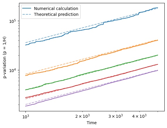
Example 2: Theoretical estiation of p-variation for FBM and p = 1/H

In the case of p = 1/H, with H being the Hurst exponent, we can theoretically calculated the value of the p-variation for an FBM process (see Eq. (6) of 1).

T = 5000
pvar_alpha = []

Hs = np.linspace(0.2,0.5,5)
pvars = []
pvars_t = []
Ds_est = []

min_idx = 1000
for idxH, H in enumerate(Hs): 

    # We create a trajectory with fixed D = 1
    traj = np.cumsum(models_phenom().disp_fbm(D = 1, alpha = H*2, T = T))
    
    pvar = p_variation(traj, p = 1/H, m = 1)
    pvar_theory = p_variation_FBM(H = H, 
                                  sigma = np.sqrt(2), # Note that definition of diffusion coefficient is different 
                                                      # for models_phenom and this function, hence introducint a sqrt(2) factor
                                  t = np.arange(T))

    plt.loglog(np.arange(T)[min_idx:], pvar[min_idx:], label = 'Numerical calculation' if idxH == 0 else '')
    plt.plot(np.arange(T)[min_idx:], pvar_theory[min_idx:], label = 'Theoretical prediction' if idxH == 0 else '',
             c = f'C{idxH}', ls = '--', alpha = 0.6)
plt.legend()
plt.ylabel('p-variation (p = 1/H)')
plt.xlabel('Time')

Text(0.5, 0, 'Time')

Power spectral density

---

source

psd

 psd (traj:numpy.ndarray)

Calculates the approximate power spectral density based on scipy.periodogram

	Type	Details
traj	ndarray	Trajectory of size (T,) (i.e. 1D) or (T, dim)
Returns	tuple	(f, psd): frequencies f and power spectral density. Sizes f: (floor(T/2)), psd: (floor(T/2))

Example: from clean to noisy trajectories

In this example we show how to use the PSD and also how the noise present in the trajectories can affect this assesment. This is based on the result of “Towards a robust criterion of anomalous diffusion”, V. Sposini et al..

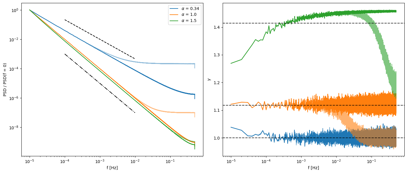
T = int(1e5)
N = int(1e4)

# Hurst exponents we will consider
Hs = np.array([1/3, 1, 3/2])/2

# Storing variables
# mean and std of the PSD for the clean trajectories
muH = np.zeros((len(Hs), int(T/2)))
stdH = np.zeros_like(muH)
# mean and std of the PSD for the noise trajectories
muH_noise = np.zeros_like(muH)
stdH_noise = np.zeros_like(muH)

sigma_noise = 1e2

for idxH, H in enumerate(tqdm(Hs)):
    
    psdH = np.zeros((N, int(T/2)))
    psdH_noise = np.zeros((N, int(T/2)))
    
    for idxN in (range(N)):
        
        # Here we generate the clean trajectories and compute their PSD
        X = models_phenom().disp_fbm(D = 1, alpha = H*2, T = T).cumsum()
        f, psd = periodogram(X)
        psdH[idxN] = psd[1:]

        # Now we noise the trajectories and compute their new PSD
        X_noise = X + np.random.randn(X.shape[0])*np.sqrt(sigma_noise)
        _, psd_noise = periodogram(X_noise)
        psdH_noise[idxN] = psd_noise[1:]

    
    muH[idxH] = psdH.mean(0)
    stdH[idxH] = psdH.std(0)

    muH_noise[idxH] = psdH_noise.mean(0)
    stdH_noise[idxH] = psdH_noise.std(0)

We can can now show what we previously calculated. The solid lines represent the clean trajectories while the shaded ones are the noisy. The dashed line in the left plot shows the expected scaling for subdiffusive trajectories while the point-dashed one is the expected scaling for normal and superdiffusive trajectories. The dashed line in the rightmost plot show the expected theoretical convergence for each type of diffusion. See more about this in “Towards a robust criterion of anomalous diffusion”, V. Sposini et al..

fig, ax = plt.subplots(1, 2, figsize = (14,6), tight_layout = True)

for idxH, H in enumerate((Hs)):
    ax[0].loglog(f[1:], muH[idxH]/muH[idxH,0], label = fr'$\alpha$ = {np.round(H,2)*2}')
    
    ax[0].loglog(f[1:], muH_noise[idxH]/muH_noise[idxH,0], c=f'C{idxH}', alpha = 0.5)
    if idxH == 0:
        ax[0].plot(np.linspace(1e-4, 1e-2, 10), 1e-6*np.linspace(1e-4, 1e-2, 10)**(-H*2-1), c = 'k', ls = '--')
    elif idxH == 1:
        ax[0].plot(np.linspace(1e-4, 1e-2, 10), 1e-11*np.linspace(1e-4, 1e-2, 10)**(-H*2-1), c = 'k', ls = '-.')

    ax[1].semilogx(f[1:-1], stdH[idxH, :-1]/ muH[idxH, :-1])
    ax[1].semilogx(f[1:-1], stdH_noise[idxH, :-1]/ muH_noise[idxH, :-1], c=f'C{idxH}', alpha = 0.6)


for line in [1, np.sqrt(2), np.sqrt(5)/2]: ax[1].axhline(line, c='k', ls = '--', alpha = 0.8)

plt.setp(ax[0], 
         xlabel = 'f [Hz]',
         ylabel = 'PSD / PSD(f = 0)'
        )

plt.setp(ax[1], 
         xlabel = 'f [Hz]',
         ylabel = r'$\gamma$'
        )

ax[0].legend()

<matplotlib.legend.Legend>