utils_challenge

Managing data

Smoothing labels

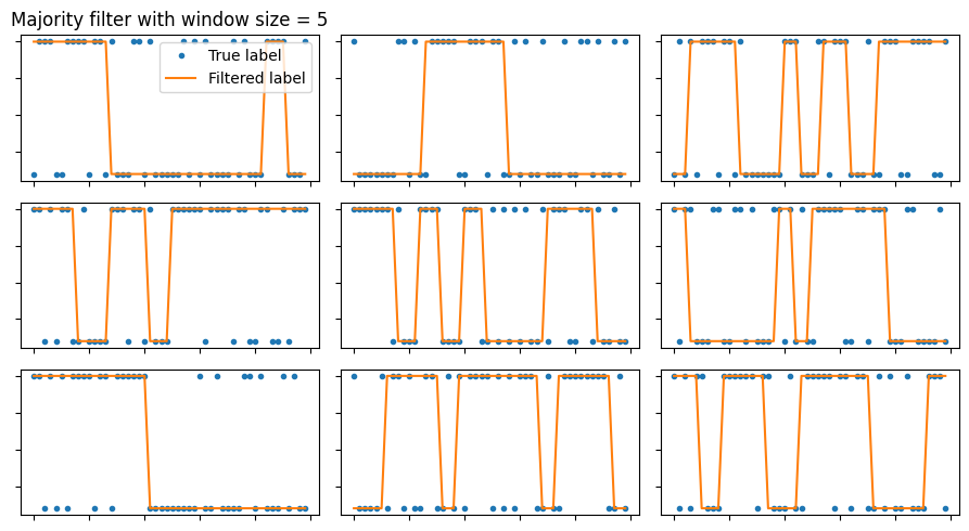
These functions are used to smooth a given vector of labels of heterogeneous processes by means of majority filter. It allows to define a minimum segment length.

---

source

label_filter

 label_filter (label, window_size=5, min_seg=3)

Given a vector of changing labels, applies a majority filter such that the minimum segment of a particular label is bigger than the minimum set segment.

	Type	Default	Details
label	list		label vector to filter.
window_size	int	5	Size of the window in which the majority filter is applied.
min_seg	int	3	Minimum segment size after filtering.
Returns	np.array		Filtered label vector

---

source

majority_filter

 majority_filter (seq, width)

Given a vector, applies a majority filter of given width.

	Type	Details
seq	list	Vector to filter.
width	int	Size of the window in which the filter is applied.
Returns	list	Filtered vector

fig, axs = plt.subplots(3, 3, figsize = (9, 5), tight_layout = True)
window_size = 5

for ax in axs.flatten():    
    traj, labs = models_phenom()._multiple_state_traj(alphas = [0.7, 0.8], Ds = [0.01, 0.1])
    filtered_d = label_filter(labs[:,1],
                              window_size = window_size)
    
    ax.plot(labs[:, 1], '.', label = 'True label')
    ax.plot(filtered_d, label = r'Filtered label')
    
axs[0,0].set_title(f'Majority filter with window size = {window_size}')
axs[0,0].legend()
plt.setp(axs, xticklabels = [], yticklabels = []);

New population percentages after filtering

Note that smoothing the signal will have an effect on the actual proportion of time a particle spends in each state. This will be taken into account in the challenge. Here we showcase this effect:

T = 100
traj, labs = models_phenom().multi_state(N = 500, alphas = [[0.7, 1],[0.4,2]], Ds = [[0, 1], [1, 0]], T = T)

res_t = np.array([])
res_ft = np.array([])
for label in tqdm(labs.transpose(1,0,2)[:,:,0]):
    
    # raw labels
    CP = np.argwhere(label[1:] != label[:-1]).flatten()
    if CP[-1] != 199: CP = np.append(CP, T-1)
    CP = np.append(0, CP)

    res_t = np.append(res_t, CP[1:] - CP[:-1])
    
    
    # filtered labels
    filt = label_filter(label)
    
    CP_f = np.argwhere(filt[1:] != filt[:-1]).flatten()
    if CP_f[-1] != 199: CP_f = np.append(CP_f, T-1)
    CP_f = np.append(0, CP_f)

    res_ft = np.append(res_ft, CP_f[1:] - CP_f[:-1])

We show now the new transition rates (e.g. 1 over the residence time of a given state). Because we are minimum segment length of 3, we can actually approximate the filtered transition rate as the original times 2/3:

print(f' True transition rate: {1/np.mean(res_t)}\n',
      f'Filtered transition rate: {1/np.mean(res_ft)}\n',
      f'True rate x 2/3: {1/np.mean(res_t)*(2/3)}')

 True transition rate: 0.10947474747474747
 Filtered transition rate: 0.07402020202020201
 True rate x 2/3: 0.07298316498316498

Continuous labels to list of features

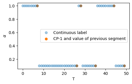
The labels in the challenge will be the list of \(n\) changepoints as well as the \(n+1\) diffusion properties (\(D\) and \(\alpha\)) for each segment. This function transforms the stepwise labels into three lists: CPs, \(\alpha\)s and \(D\)s.

---

source

label_continuous_to_list

 label_continuous_to_list (labs)

Given an array of T x 2 labels containing the anomalous exponent and diffusion coefficient at each timestep, returns 3 arrays, each containing the changepoints, exponents and coefficient, respectively. If labs is size T x 3, then we consider that diffusive states are given and also return those.

	Type	Details
labs	array	T x 2 or T x 3 labels containing the anomalous exponent, diffusion and diffusive state.
Returns	tuple	- First element is the list of change points - The rest are corresponding segment properties (order: alpha, Ds and states)

# Generate the trajectory
trajs, labels = models_phenom().multi_state(N = 1, T = 50)

# Transform the labels:
CP, alphas, Ds, _ = label_continuous_to_list(labels[:,-1,:])

plt.figure(figsize=(5, 3))
plt.plot(labels[:, -1, 1], 'o', alpha = 0.4, label = 'Continuous label')
plt.scatter(CP-1, Ds, c = 'C1', label = 'CP-1 and value of previous segment')
plt.legend(); plt.xlabel('T'); plt.ylabel(r'$\alpha$')

Text(0, 0.5, '$\\alpha$')

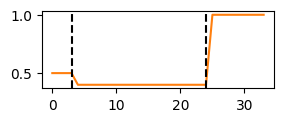
List of features to continuous labels

This function does the opposite from than label_continuous_to_list. From a list of properties as the one used in ANDI 2 challenge, creates continuous labels.

---

source

label_list_to_continuous

 label_list_to_continuous (CP, label)

Given a list of change points and the labels of the diffusion properties of the resulting segments, generates and array of continuous labels. The last change point indicates the array length.

	Type	Details
CP	array, list	list of change points. Last change point indicates label length.
label	array, list	list of segment properties
Returns	array	Continuous label created from the given change points and segment properties

CP = [3,24,34]
label = [0.5, 0.4, 1]
cont = label_list_to_continuous(CP, label)
plt.figure(figsize = (3,1))
plt.plot(cont, c = 'C1')
[plt.axvline(c, c = 'k', ls = '--') for c in CP[:-1]];

Storing array data in dataframe

---

source

array_to_df

 array_to_df (trajs, labels, min_length=10, fov_origin=[0, 0],
              fov_length=100.0, cutoff_length=10)

Given arrays for the position and labels of trajectories, creates a dataframe with that data. The function also applies the demanded FOV. If you don’t want a field of view, chose a FOV length bigger (smaller) that your maximum (minimum) trajectory position.

	Type	Default	Details
trajs	array		Trajectories to store in the df (dimension: T x N x 3)
labels	array		Labels to store in the df (dimension: T x N x 3)
min_length	int	10
fov_origin	list	[0, 0]	Bottom left point of the square defining the FOV.
fov_length	float	100.0	Size of the box defining the FOV.
cutoff_length	int	10	Minimum length of a trajectory inside the FOV to be considered in the output dataset.
Returns	tuple		- df_in (dataframe): dataframe with trajectories - df_out (datafram): dataframe with labels

#trajs, labels = models_phenom().multi_state(T = 200, N = 10, alphas=[0.5, 1], Ds = [1,1], L = 100)
trajs, labels = models_phenom().single_state(T = 200, N = 10)

# Changing dimensions
trajs = trajs.transpose((1, 0, 2)).copy()
labels = labels.transpose(1, 0, 2)

df_in, df_out = array_to_df(trajs, labels)

df_out.head()

	traj_idx	Ds	alphas	states	changepoints
0	0	[1.0]	[1.0]	[2.0]	[115]
1	1	[1.0]	[1.0]	[2.0]	[22]
2	2	[1.0]	[1.0]	[2.0]	[10]
3	3	[1.0]	[1.0]	[2.0]	[39]
4	4	[1.0]	[1.0]	[2.0]	[28]

Transform ANDI dataframe to array with padding

---

source

df_to_array

 df_to_array (df, pad=-1)

Transform a dataframe as the ones given in the ANDI 2 challenge (i.e. 4 columns: traj_idx, frame, x, y) into a numpy array. To deal with irregular temporal supports, we pad the array whenever the trajectory is not present. The output array has the typical shape of ANDI datasets: TxNx2

	Type	Default	Details
df	dataframe		Dataframe with four columns ‘traj_idx’: the trajectory index, ‘frame’ the time frame and ‘x’ and ‘y’ the positions of the particle.
pad	int	-1	Number to use as padding.
Returns	array		Array containing the trajectories from the dataframe, with usual ANDI shape (TxNx2).

Reorganize folder for challenge if non-overlapping FOVS

The outputs of datasets_challenge.challenge_phenom_dataset are not in the appropriate form if one considers the case of non-overlapping FOVS. The latter means that instead of taking n_fovs from the same experiment, we repeat the same experiment n_fovs times. This functions rearranges the folders to get the proper structure proposed in the paper.

---

source

file_nonOverlap_reOrg

 file_nonOverlap_reOrg (raw_folder, target_folder, experiments, num_fovs,
                        tracks=[1, 2], save_labels=False, task=['single',
                        'ensemble'], print_percentage=True)

This considers that you have n_fovs*n_experiments ‘fake’ experiments and organize them based on the challenge instructions

	Type	Default	Details
raw_folder			original folder with data produced by datasets_challenge.challenge_phenom_dataset
target_folder
experiments
num_fovs
tracks	list	[1, 2]
save_labels	bool	False	If True, moves all data (also labels,.. etc). Do True only if saving reference / groundtruth data
task	list	[‘single’, ‘ensemble’]
print_percentage	bool	True

Isolate VIP particles

---

source

get_VIP

 get_VIP (array_trajs, num_vip=5, min_distance_part=2, pad=-1,
          boundary=False, boundary_origin=(0, 0), min_distance_bound=0,
          sort_length=True)

Given an array of trajectories, finds the particles VIP particles that participants will need to characterize in the video trakcl.

The function first finds the particles that exist at frame 0 (i.e. that their first value is different from pad). Then, iterates over this particles to find num_vip that are at distance > than min_distance_part in the first frame.

	Type	Default	Details
array_trajs	array		Position of the trajectories that will be considered for the VIP search.
num_vip	int	5	Number of VIP particles to flag.
min_distance_part	int	2	Minimum distance between two VIP particles.
pad	int	-1	Number used to indicate in the temporal support that the particle is outside of the FOV.
boundary	bool	False	If float, defines the length of the box acting as boundary
boundary_origin	tuple	(0, 0)	X and Y coords of the boundary
min_distance_bound	int	0	Minimum distance a particles has to be from the boundary in ordered to be considered a VIP particle
sort_length	bool	True	If True, candidates for VIP particles are choosen in descending trajectory length. This ensures that the longest ones are chosen.
Returns	list		List of indices of the chosen VIP particles

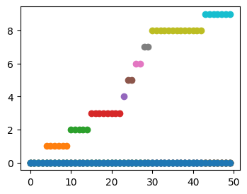
# define random trajectories
array_trajs = np.random.rand(200,10, 2)*10
# insert paddings to make first trajectories finish earlier
pad = -1
array_trajs[100, :,:] = pad
array_trajs[0,3,0] = pad
array_trajs.shape

(200, 10, 2)

get_VIP(array_trajs, num_vip = 5, min_distance_part = 0, pad = pad, 
        boundary = 10, boundary_origin = (0,0), min_distance_bound = 0,
        sort_length = True)

[0, 1, 2, 4, 5]

ANDI 2 challenge metrics

Setting maximum erros for different metrics

Changepoint pairing

We use an assignment algorithm to pair predicted and groundtruth changepoints. From there, we will calculate the various metrics of the challenge.

---

source

changepoint_assignment

 changepoint_assignment (GT, preds)

Given a list of groundtruth and predicted changepoints, solves the assignment problem via the Munkres algorithm (aka Hungarian algorithm) and returns two arrays containing the index of the paired groundtruth and predicted changepoints, respectively.

The distance between change point is the Euclidean distance.

	Type	Details
GT	list	List of groundtruth change points.
preds	list	List of predicted change points.
Returns	tuple	- tuple of two arrays, each corresponding to the assigned GT and pred changepoints - Cost matrix

ngts = 10; npreds = 6; T = 100
GT = np.sort(np.random.choice(np.arange(1,T), ngts, replace = False))
preds = np.sort(np.random.choice(np.arange(1,T)*0.5, npreds, replace = False)).astype(int)
print('GT:', GT)
print('Pred:', preds)
changepoint_assignment(GT, preds)[0]

GT: [ 2  8 24 33 34 54 55 64 73 85]
Pred: [ 8 11 16 30 36 47]

(array([0, 1, 2, 3, 4, 5], dtype=int64),
 array([1, 0, 2, 3, 4, 5], dtype=int64))

---

source

changepoint_alpha_beta

 changepoint_alpha_beta (GT, preds, threshold=10)

Calculate the alpha and beta measure of paired changepoints. Inspired from Supplemantary Note 3 in https://www.nature.com/articles/nmeth.2808

	Type	Default	Details
GT	list		List of groundtruth change points.
preds	list		List of predicted change points.
threshold	int	10	Distance from which predictions are considered to have failed. They are then assigned this number.
Returns	tuple		alpha, beta

labels = [r'Random Guess + $N_p>N_{gt}$',
          r'Random Guess + $N_p<N_{gt}$',
          r'GT + rand $\in [-3, 3]$',
          r'GT + rand $\in [-1, 1]$']

fig, ax = plt.subplots(figsize = (4,3))
alpha = 0.2

T = 200; ngts = 15; 

for case, (label, color) in enumerate(zip(labels, ['C0', 'C1', 'C2', 'C3'])):

    alphas, betas = [], []
    for _ in range(100):
        
        GT = np.sort(np.random.choice(np.arange(1,T), ngts, replace = False))
        if case == 0:
            npreds = np.random.randint(low = ngts, high = ngts*2)
            preds = np.sort(np.random.choice(np.arange(1,T), npreds, replace = False)) 
        elif case == 1:
            npreds = np.random.randint(low = 1, high = ngts)
            preds = np.sort(np.random.choice(np.arange(1,T), npreds, replace = False))     
        elif case == 2:
            preds = GT + np.random.randint(-3, 3, ngts)
        elif case == 3:
            preds = GT + np.random.randint(-1, 1, ngts)
            
        alpha, beta = changepoint_alpha_beta(GT, preds)
        
        alphas.append(alpha)
        betas.append(beta)
     
    
    ax.scatter(alphas, betas, c = color, alpha = alpha)
    ax.scatter(np.mean(alphas), np.mean(betas), c = color, label = label, s = 50, marker = 's', edgecolors = 'k')
plt.setp(ax, xlabel = r'$\alpha$', ylabel = r'$\beta$')
ax.legend(loc = (1.01,0.4))

<matplotlib.legend.Legend>

---

source

jaccard_index

 jaccard_index (TP:int, FP:int, FN:int)

Given the true positive, false positive and false negative rates, calculates the Jaccard Index

	Type	Details
TP	int	true positive
FP	int	false positive
FN	int	false negative
Returns	float	Jaccard Index

---

source

single_changepoint_error

 single_changepoint_error (GT, preds, threshold=5)

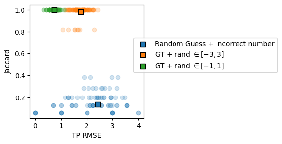
Given the groundtruth and predicted changepoints for a single trajectory, first solves the assignment problem between changepoints, then calculates the RMSE of the true positive pairs and the Jaccard index.

	Type	Default	Details
GT	list		List of groundtruth change points.
preds	list		List of predicted change points.
threshold	int	5	Distance from which predictions are considered to have failed. They are then assigned this number.
Returns	tuple		- TP_rmse: root mean square error of the true positive change points. - Jaccard Index of the ensemble predictions

---

source

ensemble_changepoint_error

 ensemble_changepoint_error (GT_ensemble, pred_ensemble, threshold=5)

Given an ensemble of groundtruth and predicted change points, iterates over each trajectory’s changepoints. For each, it solves the assignment problem between changepoints. Then, calculates the RMSE of the true positive pairs and the Jaccard index over the ensemble of changepoints (i.e. not the mean of them w.r.t. to the trajectories)

	Type	Default	Details
GT_ensemble	list, array		Ensemble of groutruth change points.
pred_ensemble	list		Ensemble of predicted change points.
threshold	int	5	Distance from which predictions are considered to have failed. They are then assigned this number.
Returns	tuple		- TP_rmse: root mean square error of the true positive change points. - Jaccard Index of the ensemble predictions

labels = ['Random Guess + Incorrect number',
          r'GT + rand $\in [-3, 3]$',
          r'GT + rand $\in [-1, 1]$']

fig, ax = plt.subplots(figsize = (3,3))
alpha = 0.2

T = 200; ngts = 10; npreds = 8

for case, (label, color) in enumerate(zip(labels, ['C0', 'C1', 'C2'])):
    
    rmse, ji = [], []
    GT, preds = [], []
    for _ in range(100):

        GT.append(np.sort(np.random.choice(np.arange(1,T), ngts, replace = False)))
        if case == 0:
            preds.append(np.sort(np.random.choice(np.arange(1,T), npreds, replace = False)))                  
        elif case == 1:
            preds.append(GT[-1] + np.random.randint(-3, 3, ngts))
        elif case == 2:
            preds.append(GT[-1] + np.random.randint(-1, 1, ngts))

        assignment, _ = changepoint_assignment(GT[-1], preds[-1])
        assignment = np.array(assignment)

        RMSE, JI = single_changepoint_error(GT[-1], preds[-1], threshold = 5)     
        
        rmse.append(RMSE)
        ji.append(JI)

    rmse_e, ji_e = ensemble_changepoint_error(GT, preds, threshold = 5)
    
    ax.scatter(rmse, ji, c = color, alpha = alpha)
    ax.scatter(rmse_e, ji_e, c = color, label = label, s = 50, marker = 's', edgecolors = 'k')
plt.setp(ax, xlabel = 'TP RMSE', ylabel = 'Jaccard')
ax.legend(loc = (0.91,0.4))

<matplotlib.legend.Legend>

Segments pairing

Here we focus on pairing the segments arising from a list of changepoints. We will use this to latter compare the predicted physical properties for each segment

---

source

create_binary_segment

 create_binary_segment (CP:list, T:int)

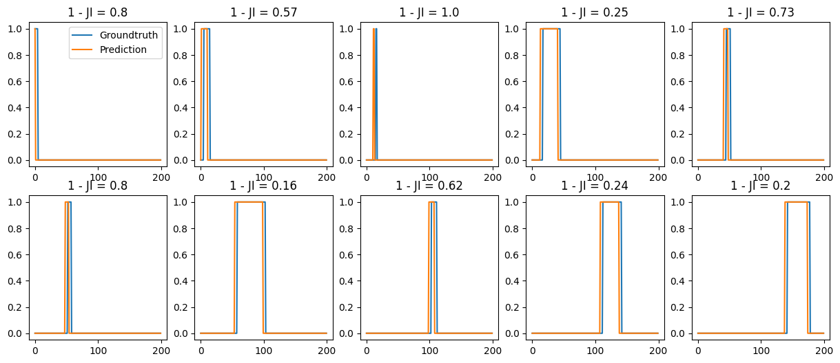
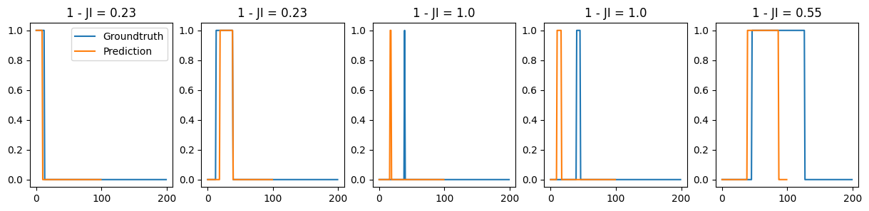
Given a set of changepoints and the lenght of the trajectory, create segments which are equal to one if the segment takes place at that position and zero otherwise.

	Type	Details
CP	list	list of changepoints
T	int	length of the trajectory
Returns	list	list of arrays with value 1 in the temporal support of the current segment.

T= 50
GT = np.sort(np.random.choice(np.arange(1,T), 10, replace = False))
plt.figure(figsize = (4,3))
for idx, x in enumerate(create_binary_segment(GT, T)):
    plt.plot(x*idx, 'o')

---

source

jaccard_between_segments

 jaccard_between_segments (gt, pred)

Given two segments, calculates the Jaccard index between them by considering TP as correct labeling, FN as missed events and FP leftover predictions.

	Type	Details
gt	array	groundtruth segment, equal to one in the temporal support of the given segment, zero otherwise.
pred	array	predicted segment, equal to one in the temporal support of the given segment, zero otherwise.
Returns	float	Jaccard index between the given segments.

---

source

segment_assignment

 segment_assignment (GT, preds, T:int=None)

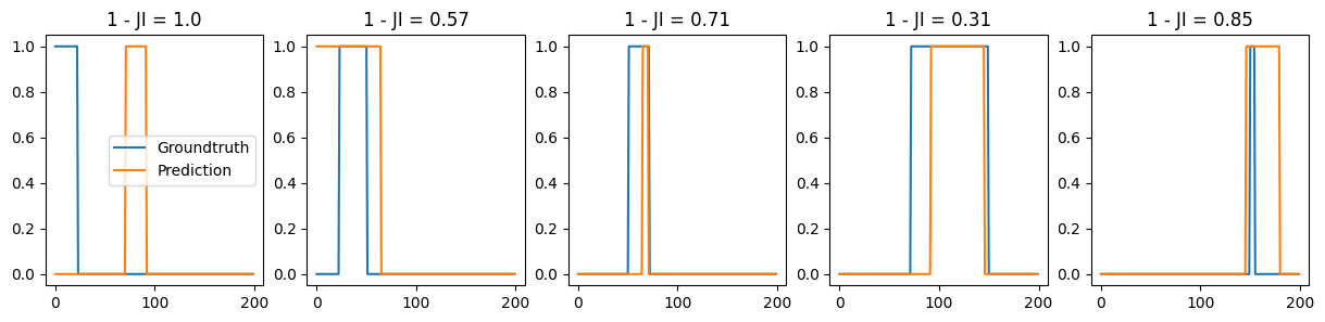
Given a list of groundtruth and predicted changepoints, generates a set of segments. Then constructs a cost matrix by calculting the Jaccard Index between segments. From this cost matrix, we solve the assignment problem via the Munkres algorithm (aka Hungarian algorithm) and returns two arrays containing the index of the groundtruth and predicted segments, respectively.

If T = None, then we consider that GT and preds may have different lenghts. In that case, the end of the segments is the the last CP of each set of CPs.

	Type	Default	Details
GT	list		List of groundtruth change points.
preds	list		List of predicted change points.
T	int	None	Length of the trajectory. If None, considers different GT and preds length.
Returns	tuple		- tuple of two arrays, each corresponding to the assigned GT and pred changepoints - Cost matrix calculated via JI of segments

Examples

Predictions close to groundtruth

T = 200; 
ngts = 10; 
GT = np.sort(np.random.choice(np.arange(1,T), ngts, replace = False))
preds = np.sort(GT + np.random.randint(-5, 5, 1) )

seg_GT = create_binary_segment(GT, T)
seg_preds = create_binary_segment(preds, T)   

[row_ind, col_ind], cost_matrix = segment_assignment(GT, preds, T)

fig, axs = plt.subplots(2, 5, figsize = (15, 6))
for r, c, ax in zip(row_ind, col_ind, axs.flatten()):
    ax.set_title(f'1 - JI = {np.round(cost_matrix[r, c], 2)}')
    ax.plot(seg_GT[r], label = 'Groundtruth')
    ax.plot(seg_preds[c], label = 'Prediction')
axs[0,0].legend()

<matplotlib.legend.Legend>

Different size between predictions and trues

T1 = 200; T2 = 100
ngts = 10; 
GT = np.sort(np.random.choice(np.arange(1,T1), ngts, replace = False))
preds = np.sort(np.random.choice(np.arange(1,T2), 5, replace = False))

seg_GT = create_binary_segment(GT, T1)
seg_preds = create_binary_segment(preds, T2)   

[row_ind, col_ind], cost_matrix = segment_assignment(GT, preds)

fig, axs = plt.subplots(1, 5, figsize = (15, 3))
for r, c, ax in zip(row_ind, col_ind, axs.flatten()):
    ax.set_title(f'1 - JI = {np.round(cost_matrix[r, c], 2)}')
    ax.plot(seg_GT[r], label = 'Groundtruth')
    ax.plot(seg_preds[c], label = 'Prediction')
axs[0].legend()

<matplotlib.legend.Legend>

Predictions very different to groundtruth

T = 200;
ngts = 5; npreds = 5;
GT = np.sort(np.random.choice(np.arange(1,T), ngts, replace = False))
preds = np.sort(np.random.choice(np.arange(1,T), npreds, replace = False))  

seg_GT = create_binary_segment(GT, T)
seg_preds = create_binary_segment(preds, T)

[row_ind, col_ind], cost_matrix = segment_assignment(GT, preds, T)

fig, axs = plt.subplots(1, 5, figsize = (15, 3))
for r, c, ax in zip(row_ind, col_ind, axs.flatten()):
    ax.set_title(f'1 - JI = {np.round(cost_matrix[r, c], 2)}')
    ax.plot(seg_GT[r], label = 'Groundtruth')
    ax.plot(seg_preds[c], label = 'Prediction')
axs[0].legend()

<matplotlib.legend.Legend>

Segment properties comparison

We use the segment pairing functions that we have defined above to compute various metrics between the properties of predicted and groundtruth segments.

Metrics of segment properties

---

source

metric_diffusive_state

 metric_diffusive_state (gt=None, pred=None)

Compute the F1 score between diffusive states.

---

source

metric_diffusion_coefficient

 metric_diffusion_coefficient (gt=None, pred=None, threshold_min=1e-12,
                               max_error=190.86835960820298)

Compute the mean squared log error (msle) between diffusion coefficients. Checks the current bounds of diffusion from models_phenom to calculate the maximum error.

---

source

metric_anomalous_exponent

 metric_anomalous_exponent (gt=None, pred=None, max_error=1.999)

Compute the mean absolute error (mae) between anomalous exponents. Checks the current bounds of anomalous exponents from models_phenom to calculate the maximum error.

x = np.random.rand(100)
y = np.random.rand(100)

metric_diffusion_coefficient(x+2,y+2, threshold_min=-2)

0.014261449910975834

Pairing and metrics calculation

---

source

check_no_changepoints

 check_no_changepoints (GT_cp, GT_alpha, GT_D, GT_s, preds_cp,
                        preds_alpha, preds_D, preds_s, T:bool|int=None)

Given predicionts over changepoints and variables, checks if in both GT and preds there is an absence of change point. If so, takes that into account to pair variables.

	Type	Default	Details
GT_cp	list, int, float		Groundtruth change points
GT_alpha	list, float		Groundtruth anomalous exponent
GT_D	list, float		Groundtruth diffusion coefficient
GT_s	list, float		Groundtruth diffusive state
preds_cp	list, int, float		Predicted change points
preds_alpha	list, float		Predicted anomalous exponent
preds_D	list, float		Predicted diffusion coefficient
preds_s	list, float		Predicted diffusive state
T	bool | int	None	(optional) Length of the trajectories. If none, last change point is length.
Returns	tuple		- False if there are change points. True if there were missing change points. - Next three are either all Nones if change points were detected, or paired exponents, coefficient and states if some change points were missing.

---

source

segment_property_errors

 segment_property_errors (GT_cp, GT_alpha, GT_D, GT_s, preds_cp,
                          preds_alpha, preds_D, preds_s,
                          return_pairs=False, T=None)

Given predicionts over change points and the value of diffusion parameters in the generated segments, computes the defined metrics.

	Type	Default	Details
GT_cp	list, int, float		Groundtruth change points
GT_alpha	list, float		Groundtruth anomalous exponent
GT_D	list, float		Groundtruth diffusion coefficient
GT_s	list, float		Groundtruth diffusive state
preds_cp	list, int, float		Predicted change points
preds_alpha	list, float		Predicted anomalous exponent
preds_D	list, float		Predicted diffusion coefficient
preds_s	list, float		Predicted diffusive state
return_pairs	bool	False	If True, returns the assigment pairs for each diffusive property.
T	NoneType	None	(optional) Length of the trajectories. If none, last change point is length.
Returns	tuple		- if return_pairs = True, returns the assigned pairs of diffusive properties - if return_pairs = False, returns the errors for each diffusive property

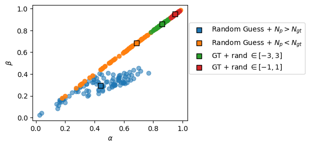
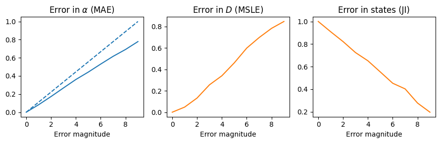
We generate some random predictions to check how the metrics behave. We consider errors also in the change point predictions, hence there will be some segment mismatchings, which will affect the diffusive properties predictions:

T = 200; 
ngts = 10; 
errors_alpha = np.linspace(0, 1, ngts)
errors_d = np.linspace(0, 10, ngts)
errors_s = np.linspace(0, 1, ngts)

metric_a, metric_d, metric_s = [], [], []
for error_a, error_d, error_s in zip(errors_alpha, errors_d, errors_s):
    la, ld, ls = [], [], []
    for _ in range(100):

        GT_cp = np.sort(np.random.choice(np.arange(1,T-1), ngts, replace = False))
        preds_cp = np.sort(np.random.choice(np.arange(1,T-1), ngts, replace = False)) 

        GT_alpha = np.random.rand(GT_cp.shape[0]+1)
        preds_alpha = GT_alpha + np.random.randn(preds_cp.shape[0]+1)*error_a

        GT_D = np.abs(np.random.randn(GT_cp.shape[0]+1)*10)
        preds_D = GT_D + np.abs(np.random.randn(preds_cp.shape[0]+1))*error_d
        
        GT_s = np.random.randint(0, 5, GT_cp.shape[0]+1)
        coin = np.random.rand(len(GT_s))
        preds_s = GT_s.copy()
        preds_s[coin < error_s] = np.random.randint(0, 5, len(coin[coin < error_s]))

        m_a, m_d, m_s = segment_property_errors(GT_cp, GT_alpha, GT_D, GT_s, preds_cp, preds_alpha, preds_D, preds_s, T = T)
        
        la.append(m_a); ld.append(m_d); ls.append(m_s)
    
    metric_a.append(np.mean(la))
    metric_d.append(np.mean(ld))    
    metric_s.append(np.mean(ls))

With no error in the changepoint predicitions:

fig, ax = plt.subplots(1, 3, figsize = (9, 3), tight_layout = True)

ax[0].plot(np.arange(ngts), errors_alpha, c = 'C0', ls = '--', label = 'Expected with no assigment error')
ax[0].plot(np.arange(ngts), metric_a, c = 'C0')
ax[0].set_title(r'Error in $\alpha$ (MAE)')

#ax[1].plot(np.arange(ngts), errors_d, c = 'C1', ls = '--')
ax[1].plot(np.arange(ngts), metric_d, c = 'C1')
ax[1].set_title(r'Error in $D$ (MSLE)')

ax[2].plot(np.arange(ngts), metric_s, c = 'C1')
ax[2].set_title(r'Error in states (JI)')

plt.setp(ax, xlabel = 'Error magnitude')

[Text(0.5, 0, 'Error magnitude'),
 Text(0.5, 0, 'Error magnitude'),
 Text(0.5, 0, 'Error magnitude')]

With error in the changepoint predicitions:

fig, ax = plt.subplots(1, 3, figsize = (9, 3), tight_layout = True)

ax[0].plot(np.arange(ngts), errors_alpha, c = 'C0', ls = '--', label = 'Expected with no assigment error')
ax[0].plot(np.arange(ngts), metric_a, c = 'C0')
ax[0].set_title(r'Error in $\alpha$ (MAE)')

#ax[1].plot(np.arange(ngts), errors_d, c = 'C1', ls = '--')
ax[1].plot(np.arange(ngts), metric_d, c = 'C1')
ax[1].set_title(r'Error in $D$ (MSLE)')

ax[2].plot(np.arange(ngts), metric_s, c = 'C1')
ax[2].set_title(r'Error in states (JI)')

plt.setp(ax, xlabel = 'Error magnitude')

[Text(0.5, 0, 'Error magnitude'),
 Text(0.5, 0, 'Error magnitude'),
 Text(0.5, 0, 'Error magnitude')]

Ensemble metrics

Get ensemble information

---

source

extract_ensemble

 extract_ensemble (state_label, dic)

Given an array of the diffusive state and a dictionary with the diffusion information, returns a summary of the ensemble properties for the current dataset.

	Type	Details
state_label	array	Array containing the diffusive state of the particles in the dataset. For multi-state and dimerization, this must be the number associated to the state (for dimerization, 0 is free, 1 is dimerized). For the rest, we follow the numeration of models_phenom().lab_state.
dic	dict	Dictionary containing the information of the input dataset.
Returns	array	Matrix containing the ensemble information of the input dataset. It has the following shape: |mu_alpha1 mu_alpha2 … | |sigma_alpha1 sigma_alpha2 … | |mu_D1 mu_D1 … | |sigma_D1 sigma_D2 … | |counts_state1 counts_state2 … |

Generate distribution and distances

---

source

multimode_dist

 multimode_dist (params, weights, bound, x, normalized=False,
                 min_var=1e-09)

Generates a multimodal distribution with given parameters. Also accounts for single mode if weight is float or int.

	Type	Default	Details
params	list		Mean and variances of every mode.
weights	list, float		Weight of every mode. If float, we consider a single mode.
bound	tuple		Bounds (min, max) of the functions support.
x	array		Support upon which the distribution is created.
normalized	bool	False
min_var	float	1e-09

# True distribution
x = np.logspace(np.log10(models_phenom().bound_D[0]), 
                      np.log10(models_phenom().bound_D[1]), 100)
weights = [0.0005,0.9]
params_true = [[0.0,0],[1.5,0.5]]
true = multimode_dist(params_true, weights, bound = models_phenom().bound_D, x = x, normalized = False, min_var=1e-9)
plt.semilogx(x, true)

---

source

distribution_distance

 distribution_distance (p:<built-infunctionarray>, q:<built-
                        infunctionarray>, x:<built-infunctionarray>=None,
                        metric='wasserstein')

Calculates distance between two distributions.

	Type	Default	Details
p	array		distribution 1
q	array		distribution 2
x	array	None	support of the distributions (not needed for MAE)
metric	str	wasserstein	distance metric (either ‘wasserstein’ or ‘mae’)
Returns	float		distance between distributions

Tests distance

Normal scenario

means = np.linspace(0, 2, 30)
normalize = False
fig = plt.figure(figsize=(15, 4))
gs = fig.add_gridspec(2, 10)

# True distribution
x = np.arange(0, 3, 0.01)
params = [[1.7,0.01]]
weights = [1]
true = multimode_dist(params, weights, bound = [0, 3], x = x, normalized = normalize)

range_x = (1,2)
idx_range = np.argwhere((x>range_x[0]) & (x<range_x[1])).flatten()


MSE = []
wass = []
for idx, mean in enumerate(means):
    params = [[mean, 0.01]]
    weights = [1]
    pred = multimode_dist(params, weights, bound = [0, 3], x = x, normalized = normalize)  
    MSE.append(distribution_distance(true, pred, metric = 'mae'))  
    wass.append(distribution_distance(true, pred, x))  
    
    if idx % 3 == 0:
        
        ax = fig.add_subplot(gs[0, int(idx/3)])
        ax.plot(x, true, label = 'True')
        ax.plot(x, pred, label = 'Predicted')        
        plt.setp(ax, yticks = []);
        
      
    if idx == 0:
        ax.legend()
        
    ax.axvline(range_x[0])
    ax.axvline(range_x[1])
    
ax_dist = fig.add_subplot(gs[1, :])
ax_dist.plot(MSE, '-o', label = 'MAE')
ax_dist.plot(wass, '-o', label = 'wasserstein')
ax_dist.legend()
plt.setp(ax_dist, ylabel = 'MAE')
ax_dist.grid()

Having a variance = 0 (as in immobile)

Wasserstein:

means = np.linspace(0, 2, 30)
normalize = False

fig = plt.figure(figsize=(15, 7))
gs = fig.add_gridspec(4, 10)

# True distribution
x = np.arange(0, 3, 0.01)
weights = [0.3, 0.9]

params_var0 = [[0,0.0],[1,0.1]]
true_var0 = multimode_dist(params_var0, weights, bound = [0, 3], x = x, normalized = normalize)

params = [[0,0.1],[1,0.1]]
true = multimode_dist(params, weights, bound = [0, 3], x = x, normalized = normalize)

wass_var0 = []
wass = []
mae_var0 = []
mae = []
for idx, mean in enumerate(means):
    params = [[mean, 0.01]]
    weights = [1]
    pred = multimode_dist(params, weights, bound = [0, 3], x = x, normalized = normalize)  
    wass_var0.append(distribution_distance(true_var0, pred, x))  
    wass.append(distribution_distance(true, pred, x))  
    
    mae_var0.append(distribution_distance(true_var0, pred, metric = 'mae'))  
    mae.append(distribution_distance(true, pred, metric = 'mae'))  
    
    if idx % 3 == 0:
        
        ax0 = fig.add_subplot(gs[0, int(idx/3)])
        ax0.plot(x, np.log(true_var0), label = 'log(True)', c = 'C0')
        ax0.plot(x, pred, label = 'Predicted', c = 'k')        
        plt.setp(ax0, yticks = [], ylim = (-5, 5));
        
        ax = fig.add_subplot(gs[1, int(idx/3)])
        ax.plot(x, true, label = 'True', c = 'C1')
        ax.plot(x, pred, label = 'Predicted', c = 'k')        
        plt.setp(ax, yticks = []);
        
      
    if idx == 0:
        ax0.legend()
        ax.legend()

ax_wass = fig.add_subplot(gs[2, :])
ax_wass.plot(wass_var0, '-o', label = 'Var_0 = 0')
ax_wass.plot(wass, '-o', label = r'Var_0 $\neq$ 0')
ax_wass.legend()
ax_wass.set_ylabel('wass dist')

ax_mse = fig.add_subplot(gs[3, :])
ax_mse.plot(mae_var0, '-o', label = 'Var_0 = 0')
ax_mse.plot(mae, '-o', label = r'Var_0 $\neq$ 0')
ax_mse.set_yscale('log')
ax_mse.set_ylabel('mse dist')

# ax_dist.grid()

Text(0, 0.5, 'mse dist')

Checking how variance of predicted affects Wasserstein distance:

variances = np.logspace(-12, -1,300)
# True distribution
x = np.logspace(-12, 1, 10000)
weights = [1]
params_true = [[0.0,0]]
true = multimode_dist(params_true, weights, bound = [1e-9, 3], x = x, normalized = normalize, min_var=1e-7)

dist = []
for idx, var in enumerate(variances):
    params = [[0.5, var]]
    weights = [1]
    pred = multimode_dist(params, weights, bound = [1e-9, 3], x = x, normalized = normalize, min_var=1e-7)  
    dist.append(distribution_distance(true, pred, x=x))  
    
plt.plot(variances, np.array(dist)+1, 'o')
plt.axvline(params_true[0][1], c = 'k', label = 'True variance')
plt.legend()
plt.xscale('log')
plt.yscale('log')

plt.xlabel('Variance prediction')
plt.ylabel('Wasserstein distance')

Text(0, 0.5, 'Wasserstein distance')

Checking if we are considering a peak at 0

# True distribution
x = np.logspace(np.log10(models_phenom().bound_D[0]), 
                      np.log10(models_phenom().bound_D[1]), 100)
weights = [0.0005,0.9]
params_true = [[0.0,0],[1.5,0.5]]
true = multimode_dist(params_true, weights, bound = models_phenom().bound_D, x = x, normalized = normalize)

plt.plot(x, true)
plt.xscale('log')

Testing maximum value of Wasserstein distance for considered \(\alpha\) and \(D\) ranges

from andi_datasets.utils_challenge import multimode_dist, distribution_distance

min_a, max_a = models_phenom().bound_alpha[0], models_phenom().bound_alpha[1]
x = np.arange(min_a, max_a, 0.01)
normalize = False

distmax = multimode_dist([[max_a,0.0001]], [1], bound = [min_a, max_a], x = x, normalized = normalize)
distmin = multimode_dist([[min_a,0.0001]], [1], bound = [min_a, max_a], x = x, normalized = normalize)

distribution_distance(distmax, distmin, x)

1.982486622823773

min_d, max_d = models_phenom().bound_D[0], models_phenom().bound_D[1]
x = np.logspace(np.log10(models_phenom().bound_D[0]), 
                      np.log10(models_phenom().bound_D[1]), 100)

distmax = multimode_dist([[max_d,0.1]], [1], bound = [min_d, max_d], x = x, normalized = normalize)
distmin = multimode_dist([[min_d,0.01]], [1], bound = [min_d, max_d], x = x, normalized = normalize)

distribution_distance(distmax, distmin, x)

-0.004896474885754287

Calculate ensemble metric

---

source

error_Ensemble_dataset

 error_Ensemble_dataset (true_data, pred_data, size_support=1000,
                         metric='wasserstein', return_distributions=False)

Calculates the ensemble metrics for the ANDI 2 challenge. The input are matrices of shape:

col1 (state 1)	col2 (state 2)	col3 (state 3)	…
\(\mu_a^1\)	\(\mu_a^2\)	\(\mu_a^3\)	…
\(\sigma_a^1\)	\(\sigma_a^2\)	\(\sigma_a^3\)	…
\(\mu_D^1\)	\(\mu_D^2\)	\(\mu_D^3\)	…
\(\sigma_D^1\)	\(\sigma_D^2\)	\(\sigma_D^3\)	…
\(N_1\)	\(N_2\)	\(N_3\)	…

	Type	Default	Details
true_data	array		Matrix containing the groundtruth data.
pred_data	array		Matrix containing the predicted data.
size_support	int	1000	size of the support of the distributions
metric	str	wasserstein	metric used to calculate distance between distributions
return_distributions	bool	False	If True, the function also outputs the generated distributions.
Returns	tuple		- distance_alpha: distance between anomalous exponents - distance_D: distance between diffusion coefficients - dists (if asked): distributions of both groundtruth and predicted data. Order: true_a, true_D, pred_a, pred_D

track = 1
# Choose the paths
PATH_PRED = f'../../testing/data/fourth_round/pred_carlo/Track{track}/'
PATH_TRUE = '../../testing/data/fourth_round/true/fourth_round/'



distance_D, distance_alpha = [], []
for exp in [2]:
    
    true = np.loadtxt(PATH_TRUE+f'exp_{exp}/ensemble_labels.txt', skiprows = 1, delimiter = ';')
    pred = np.loadtxt(PATH_PRED+f'exp_{exp}/ensemble_pred.txt', skiprows = 1, delimiter = ';')
    
    df_true = pandas.DataFrame(data = true.reshape(1,5) if exp == 1 else true.transpose(), 
                           columns = [r'mean $\alpha$', r'var $\alpha$', r'mean $D$', r'var $D$', '% residence time'])
    df_pred = pandas.DataFrame(data = pred.reshape(1,5) if exp == 1 else pred.transpose(), 
                           columns = [r'mean $\alpha$', r'var $\alpha$', r'mean $D$', r'var $D$', '% residence time'])

#     print(f'Experiment {exp}: \nGroundtruth:')
#     display(df_true)
#     print('Prediction:')
#     display(df_pred)
#     print('------ \n')

    distance_D.append(distance_D_exp)
    distance_alpha.append(distance_a_exp)
    
    distance_a_exp, distance_D_exp, dists = error_Ensemble_dataset(true, pred, return_distributions = True)


print(f'Distance distribution D = {np.mean(distance_D)}')
print(fr'Distance distribution $\alpha$ = {np.mean(distance_alpha)}')

Distance distribution D = 0.06045239400247898
Distance distribution $\alpha$ = 0.10273932574583697

Single trajectory metrics

The participants will have to output predictions in a .txt file were each line corresponds to the predictions of a trajectory. The latter have to be ordered as:

0, d\(_0\), a\(_0\), s\(_0\), t\(_1\), d\(_1\), a\(_1\), s\(_1\), t\(_2\), d\(_2\), a\(_2\), s\(_2\), …. t\(_n\), d\(_n\), a\(_n\), s\(_n\),\(T\)

where the first number corresponds to the trajectory index, then d\(_i\), a\(_i\), s\(_i\) correspond to the diffusion coefficient, anomalous exponent and diffusive state of the \(i\)-th segment. For the latter, we have the following code: - 0: immobile - 1: confined - 2: free (unconstrained) - 3: directed

Last, t\(_j\) corresponds to the \(j\)-th changepoints. The last changepoint \(T\) corresponds to the length of the trajectory. Each prediction must contain \(C\) changepoints and \(C\) segments property values. If this is not fulfilled, the whole trajectory is considered as mispredicted.

The .txt file will be first inspected. The data will then be collected into a dataframe

---

source

check_prediction_length

 check_prediction_length (pred)

Given a trajectory segments prediction, checks whether it has C changepoints and C+1 segments properties values. As it must also contain the index of the trajectory, this is summarized by being multiple of 4. In some cases, the user needs to also predict the final point of the trajectory. In this case, we will have a residu of 1.

---

source

separate_prediction_values

 separate_prediction_values (pred)

Given a prediction over trjaectory segments, extracts the predictions for each segment property as well as the changepoint values.

---

source

load_file_to_df

 load_file_to_df (path_file, columns=['traj_idx', 'Ds', 'alphas',
                  'states', 'changepoints'])

Given the path of a .txt file, extract the segmentation predictions based on the rules of the ANDI 2 challenge022

Saving fake data for test

file_gt, file_p = [], []
T = 200; ngts = 10;
for traj in range(100):
    GT_cp = np.sort(np.random.choice(np.arange(1,T), ngts, replace = False))
    preds_cp = np.sort(np.random.choice(np.arange(1,T+50), ngts, replace = False)) 

    GT_alpha = np.random.rand(GT_cp.shape[0]+1)
    preds_alpha = GT_alpha# + 0.1 #np.random.randn(preds_cp.shape[0]+1)*0.1

    GT_D = np.abs(np.random.randn(GT_cp.shape[0]+1)*10)
    preds_D = GT_D + 1.5 #np.abs(np.random.randn(preds_cp.shape[0]+1))*1.6
    
    GT_state = np.random.randint(0, high = 5, size = GT_cp.shape[0]+1)
    preds_state = np.random.randint(0, high = 5, size = preds_cp.shape[0]+1)
    
    list_gt, list_p = [traj, GT_D[0], GT_alpha[0], GT_state[0]], [traj, preds_D[0], preds_alpha[0], preds_state[0]]
    for gtc, gta, gtd, gts, pc, pa, pd, ps in zip(GT_cp, GT_alpha[1:], GT_D[1:], GT_state[1:], preds_cp, preds_alpha[1:], preds_D[1:], preds_state[1:]):
        list_gt += [gtc, gtd, gta, gts]
        list_p += [pc, pd, pa, ps]
        
    file_gt.append(list_gt)
    if traj != 6:
        file_p.append(list_p)
        
pred_path, true_path = 'pred_test.txt', 'true_test.txt'
np.savetxt(true_path, file_gt, delimiter=',')
np.savetxt(pred_path, file_p, delimiter=',')

Recovering the data

pred_path, true_path = 'pred_test.txt', 'true_test.txt'

df_pred = load_file_to_df(pred_path)
df_true = load_file_to_df(true_path)

---

source

error_SingleTraj_dataset

 error_SingleTraj_dataset (df_pred, df_true, threshold_error_alpha=None,
                           max_val_alpha=2, min_val_alpha=0,
                           threshold_error_D=None, max_val_D=1000000.0,
                           min_val_D=1e-06, threshold_error_s=None,
                           threshold_cp=None, prints=True,
                           disable_tqdm=False)

Given two dataframes, corresponding to the predictions and true labels of a set of trajectories from the ANDI 2 challenge022, calculates the corresponding metrics Columns must be for both (no order needed): traj_idx | alphas | Ds | changepoints | states df_true must also contain a column ‘T’.

	Type	Default	Details
df_pred	dataframe		Predictions
df_true	dataframe		Groundtruth
threshold_error_alpha	NoneType	None	(same for D, s, cp) Maximum possible error allowed. If bigger, it is substituted by this error.
max_val_alpha	int	2	(same for D, s, cp) Maximum value of the parameter.
min_val_alpha	int	0	(same for D, s, cp) Minimum value of the parameter.
threshold_error_D	NoneType	None
max_val_D	float	1000000.0
min_val_D	float	1e-06
threshold_error_s	NoneType	None
threshold_cp	NoneType	None
prints	bool	True
disable_tqdm	bool	False	If True, disables the progress bar.
Returns	tuple		- rmse_CP: root mean squared error change points - JI: Jaccard index change points - error_alpha: mean absolute error anomalous exponents - error_D: mean square log error diffusion coefficients - error_s: Jaccar index diffusive states

Test

Two datasets with same number of trajs

trajs, labels = models_phenom().immobile_traps(T = 200, N = 250, alphas=0.5, Ds = 1, L = 20, Nt = 100, Pb = 1, Pu = 0.5)

trajs = trajs.transpose((1, 0, 2)).copy()
labels = labels.transpose(1, 0, 2)

df_in, df_trues = array_to_df(trajs, labels)

trajs, labels = models_phenom().immobile_traps(T = 200, N = 250, alphas=[0.5, 0.1], Ds = 1, L = 20, Nt = 100, Pb = 1, Pu = 0.5)

trajs = trajs.transpose((1, 0, 2)).copy()
labels = labels.transpose(1, 0, 2)

df_in, df_preds = array_to_df(trajs, labels)

error_SingleTraj_dataset(df_preds, df_trues, prints = True, disable_tqdm=True);

Summary of metrics assesments:

Changepoint Metrics 
RMSE: 4.285 
Jaccard Index: 0.421 

Diffusion property metrics 
Metric anomalous exponent: 0.30181845745010744 
Metric diffusion coefficient: 0.22899984105532623 
Metric diffusive state: 0.5233668341708543

Two datasets with different number of trajectories

trajs, labels = models_phenom().immobile_traps(T = 200, N = 350, alphas=[0.5,0.01], Ds = [1., 0.1], L = 20, Nt = 100, Pb = 1, Pu = 0.5)

trajs = trajs.transpose((1, 0, 2)).copy()
labels = labels.transpose(1, 0, 2)

df_in, df_trues = array_to_df(trajs, labels, label_values=[0.5, 1], diff_states=[3, 2])

trajs, labels = models_phenom().immobile_traps(T = 200, N = 250, alphas=[0.5, 0.1], Ds = 1, L = 20, Nt = 100, Pb = 1, Pu = 0.5)

trajs = trajs.transpose((1, 0, 2)).copy()
labels = labels.transpose(1, 0, 2)

df_in, df_preds = array_to_df(trajs, labels, label_values=[0.5, 1], diff_states=[3, 2])

error_SingleTraj_dataset(df_preds, df_trues, prints = True)

Summary of metrics assesments:

100 missing trajectory/ies. 

Changepoint Metrics 
RMSE: 4.051 
Jaccard Index: 0.441 

Diffusion property metrics 
Metric anomalous exponent: 0.35483874584715985 
Metric diffusion coefficient: 3.1690909054732668 
Metric diffusive state: 0.4913685263947961

(4.050708208970335,
 0.4407643312101911,
 0.35483874584715985,
 3.1690909054732668,
 0.4913685263947961)

trajs, labels = models_phenom().immobile_traps(T = 200, N = 5, alphas=[0.5,0.01], Ds = [1., 0.1], L = 20, Nt = 100, Pb = 1, Pu = 0.5)

trajs = trajs.transpose((1, 0, 2)).copy()
labels = labels.transpose(1, 0, 2)

df_in, df_preds  = array_to_df(trajs, labels, label_values=[0.5, 1], diff_states=[3, 2])

trajs, labels = models_phenom().multi_state(T = 200, N = 7, L = 20, M = np.array([[0.9,0.1],[0.9,0.1]]))

trajs = trajs.transpose((1, 0, 2)).copy()
labels = labels.transpose(1, 0, 2)

df_in, df_trues  = array_to_df(trajs, labels, label_values=[0.5, 1], diff_states=[3, 2])

error_SingleTraj_dataset(df_preds, df_trues, prints = True);

Summary of metrics assesments:

2 missing trajectory/ies. 

Changepoint Metrics 
RMSE: 2.903 
Jaccard Index: 0.188 

Diffusion property metrics 
Metric anomalous exponent: 0.8269399281523714 
Metric diffusion coefficient: 8.262443034681892 
Metric diffusive state: 0.41379310344827586

Dataset with no changepoints

L = 250
# TRUES
trajs, labels = models_phenom().single_state(T = 200, N = 250, alphas=[0.5, 0.01], Ds = [1,0], L = L)
trajs = trajs.transpose((1, 0, 2)).copy()
labels = labels.transpose(1, 0, 2)

df_in, df_trues = array_to_df(trajs, labels, fov_length = L)

# PREDS
trajs, labels = models_phenom().single_state(T = 200, N = 250, L = L)

trajs = trajs.transpose((1, 0, 2)).copy()
labels = labels.transpose(1, 0, 2)

df_in, df_preds = array_to_df(trajs, labels, fov_length = L)

error_SingleTraj_dataset(df_preds, df_trues, prints = True, disable_tqdm=True);

Summary of metrics assesments:

Changepoint Metrics 
RMSE: 0 
Jaccard Index: 1 

Diffusion property metrics 
Metric anomalous exponent: 0.5025766161725703 
Metric diffusion coefficient: 0.0 
Metric diffusive state: 1.0

Codalab scoring program

Single trajectory

---

source

run_single_task

 run_single_task (exp_nums, track, submit_dir, truth_dir)

---

source

when_error_single

 when_error_single (wrn_str)

Ensemble

---

source

run_ensemble_task

 run_ensemble_task (exp_nums, track, submit_dir, truth_dir)

Parent program

---

source

codalab_scoring

 codalab_scoring (INPUT_DIR=None, OUTPUT_DIR=None)

	Type	Default	Details
INPUT_DIR	NoneType	None	directory to where to find the reference and predicted labes
OUTPUT_DIR	NoneType	None	directory where the scores will be saved (scores.txt)

---

source

listdir_nohidden

 listdir_nohidden (path)

Helpers transform results dataset in reference dataset

---

source

transform_ref_to_res

 transform_ref_to_res (base_path:str, track:str, num_fovs:int)

Transforms an organized reference dataset into a valid submission dataset. Note that we do not account for VIP indices in track_1, so will later yield an error when scoring this track.

	Type	Details
base_path	str	path where to find the folder to reorganize
track	str	either ‘track_1’ or ‘track_2’
num_fovs	int